Category Archives: Science

Questions about Mid-Month Pattern

QUESTIONS ABOUT MID-MONTH PATTERN

For much of the next week here in Wichita, we will be looking at gradually increasing temperatures and chances for storms. Will the pattern change and do we have any cool downs in store for us? Lets take a look.

Multiple waves of energy look to traverse the US through the end of this week and into the weekend. Looking at water vapor imagery this morning, you can make out multiple pieces of energy with the most organized looking system being located in the East. There is also another piece currently pushing onshore in the West. This will be what brings the Plains to Upper Midwest severe weather chances this weekend.

Zooming into this severe weather threat would show that there is a decent setup. That aforementioned wave moving onshore in the West will progress eastward, with the GFS showing its position to be titled from east Kansas through southern Minnesota Saturday evening. Coupled with upper level divergence present, these two mechanisms will provide appreciable amounts of lift to promote thunderstorm development.

With respect to moisture and how buoyant the atmosphere will be. There are a few things which are going to allow air to rise. First off, dew points in the 60s-70s coupled with diurnal heating is going to push CAPE values at least into the 1000-2000 J/kg range. Areas of higher instability will be present across southeast Kansas through south-central Iowa.

On top of this, dry air at 700 mb will continue to promote upward motion via latent heat release.

As storms develop on the front, northwesterly shear coupled with the movement of the shortwave being zonal (west to east) will push storms east-northeast. Storms will continue through the overnight into Wisconsin given the presence of a LLJ. These overnight storms could bring much needed rain to portions of northern Iowa where portions of the area are experiencing extreme drought.

Beyond Saturday, the weather will remain mostly clean through much of the next week.

The next significant chance of rain will be next weekend as a cold front attempts to push through the Central Plains. Currently, there is agreement from model output that storms will occur either Saturday or Sunday. The questions are, does the front move through and cool us down? OR do we go right back to the pattern we have been dealing with?

Looking at what the disagreement is, you can see below that the GFS has a more anomalous trough across the High Plains and Prairies while the Euro has substantial ridging setting up into the Northwest.

There are big implications here as the GFS would usher in cooler temperatures while the Euro would keep us in a similar pattern to what we’ve been seeing most of the summer (gradual warming, large cold front, gradual warming, so on so forth…). Ensembles would side with the Euro idea. The 00z GEFS mid level heights so a pattern that is more indicative of what the operation euro is putting out than what the GFS is.

Another thing to consider and monitor going forward will be the impact of the tropical Pacific on the mid level pattern across the US mid to late month. Currently, there is a storm moving up west Asia. The remnants of this storm will make its influence on the US about a week later. Perhaps the GFS is onto something here.

However, I like the placement of the blocking ridge in the northeast Pacific. There will also be multiple storms impacting the east Pacific which should act to enhance the ridge to the north.

Perhaps a blend of the Euro/GFS is what is preferred. Namely that a trough will dig into the US but will kick more into the east rather than the High Plains and Prairies. This is what the EPS hints at which means much of the same pattern moving into late August.

Good news with that is for July through August, we have been 2.8 degrees below normal. We also have only got 1.2 inches of rain which is making it dry out. This will make being outside enjoyable compared to usually being roasted out by this point in the summer.

Tropical Activity To Ramp Up Mid-Month

We’ve been in quite the stretch of quiet weather in the tropics, but there are signs that activity will quickly trend upwards later this month.

First off, why the lull?

Tropical cyclones thrive when there is divergence of mass in the upper troposphere. This allows air to efficiently rise. Late in July, much of the tropics were under upper convergence. This causes large scale downward motion. Take a look at the two images below which were analyzed on July 20th and 25th. Brown colors denote convergence and you can see quite a bit of it from Central America through the southeast Atlantic on the 20th and 25th.

That wasn’t the only thing suppressing development. Through the later half of July, there was wind shear present across much of the Caribbean. Tropical cyclones can strengthen in environments where the deep layer shear is less than 20 knots, but as you can see in the image below, the shear was as high as 50 knots.

Lastly, to get any storm to develop, you need moisture. Much of the tropical Atlantic was pestered with dry air through the later half of July. Looking at the satellite image below from the 23rd, you can see those brick red/orange colors from the Antilles through west Africa. This is dry air and it has been pushing into the Atlantic storm track, keeping thunderstorm and development potential to a minimum.

Today is August 4th and as we look forward to mid August, things are changing which could allow tropical activity to ramp up.

First, looking at our convergent wind aloft. Things continue to trend towards more upper level divergence. Examining the analysis from August 1st, you can see there is quite a bit of divergence developing in the southeast Atlantic. The only area of potential downward motion is across the Antilles.

With respect to shear, there absolutely is still some present, but the spacial area of 20 knots + is much less now than what it was in late July.

Trends would indicate that while there will be areas of shear present across the Caribbean which will act to suppress tropical activity, there won’t be enough shear to eliminate the potential with there being ample areas of favorable shear for storms to strengthen (ex. East coast, Antilles).

Last but not least, looking at moisture. The African monsoon is particularly active at the moment which is causing a deep layer of moisture to move off the continent. See the 06z GFS below.

Dry air is still in place to the north of this area but for the time being, this moisture is going to continue to be serviced by the storm activity over Africa. This is going to allow moisture to surge westward into the Caribbean, and eventually towards the Southeast US by mid month.

If one of these waves can move into a favorable shear environment then it won’t have much trouble quickly organizing, especially with such warm water present. Sea surface temperatures are ripe across the Gulf into the Florida Keys at over 30C but are plenty warm across all of the tropics.

Ensemble models are picking up on this development potential with many members outputting low centers from the Gulf through the Outer Banks mid month. All this is to say that while we have been in a lull, there is good reason not to let your guard down. Especially with us approaching the peak of tropical season.

Tropical Cyclones and Precipitation Distribution

Tropical Storm Cristobal ~June 6th, 2020

Flooding and storm surge are the two most deadly elements of a tropical cyclone (TC). In this post, I am going to explore the forecasting of heavy rain and flooding within TCs. To do this, I have read “Precipitation Distribution Associated with Landfalling Tropical Cyclones over the Eastern United States” by Eyad Atallah, Lance F. Bosart and Anantha R. Aiyyer. I plan to summarize what I believe to be the key findings from this paper, and will organize them here so they can be utilized in the operational setting.

INTRO

Before they enter their study, they talk in brief about extratropical transition (ET), how it occurs, its varying definitions depending on frameworks and what determines its strength. They note, [from Atallah and Bosart (2003)] that the distribution and intensity of rainfall depend on surrounding synoptic features (troughs/ridges) and the TC’s transition to a extratropical cyclone (EC). So when ET occurs is very important in addition to the surrounding synoptic features. ET is a complicated process and as mentioned above, it has varying definitions depending on different frameworks (QG, PV, cross sections, surface frontal boundaries). There are a few debated definitions of how ET occurs. First, changes in the low-level thickness field and mid-tropospheric thermal wind; second and more simply, look at the system and once you can identify frontal and thermal structures ET has occurred. It should be noted that while it is important to know when ET will occur, it matters little the strength of the extratropical cyclone as heavy rain events have been recorded out both weak [Hurricane Camille (1969)] and strong [Irene (1999)] ECs. As to whether the ECs will be strong or not depends mostly on whether a negatively titled trough is located upstream of a TC [Hart et al. (2006)]. If the trough is positively tilted, than a weaker EC is preferred. However, “the main focus of this paper is to understand the synoptic-scale dynamics modulating the precipitation distribution associated with landfalling TCs” (pg. 2187).

STORMS STUDIED

The 32 storms that were compiled were storms which had all of the following:

  • Landfall was along either the Gulf or Atlantic coasts of the United States.
  • The storm had to display a poleward component in its track.
  • The storm was far enough inland to permit rain measurements in all quadrants of the storm.

Some of the storms that the team analyzed are listed below with LOC meaning “left of center” and ROC meaning “right of center”. You will note that some fall under both of the LOC and the ROC composite. The times listed are when the cyclone started exhibiting that particular bias.

A list of TCs included in the study. The dates and times listed represent the initial time that a storm was included in each of the composites. The numbers in parentheses show the maximum sustained wind (kt) of the cyclone at the time listed as taken from the best-track data.

RESULTS

The storm tracks which produced the LOC and ROC composites are below.

The tracks of the tropical cyclones (based on the National Hurricane Center best-track data) for (a) storms with precipitation to the left of track and (b) storms with precipitation to the right of track.

With the LOC tracks, notice that there is a pretty broad spectrum of tracks with respect to spacial area covered. This is to say that while the Appalachians and cold air damming (CAD) will influence precipitation distribution, it is not necessary for a LOC event to occur as they occur to the east and west of the Apps. At the same time however, do note that the LOC tracks which make landfall farther north align with the LOC composite rather than the ROC tracks. This is to say that storm tracks which landfall farther north will be more heavily influenced by CAD and mid-level troughs which make heavy precipitation LOC more likely. With the ROC tracks, notice that all storms that made landfall on the east coast which exhibited ROC characteristics made landfall between Georgia and South Carolina. The rest of the tracks made landfall across the Gulf. Note that tracks which push farther into the Mississippi Valley are more likely to be ROC while most of the LOC tracks are farther east.

SYNOPTIC OVERVIEW

The 1000–500-hPa thickness (dashed black lines, contoured every 60 m), 1000-hPa geopotential height (solid black lines, contoured every 30 m), and the 850–200-hPa wind shear (shaded, contoured every 5 m s−1, starting at 20 m s−1) for (a) LOC at t = 0, (b) LOC at t = 12, (c) LOC at t = 24, (d) ROC at t = 0, (e) ROC at t = 12, and (f) ROC at t = 24. Thick solid lines denote thermal trough axes. The thick arrows in (a) and (d) depict the composite storm tracks.

The above figure has 1000-500 mb thickness in dashed lines, 1000 mb heights in solid lines and 850-200 mb shear in m/s filled. The LOC is on the left while the ROC composite is on the right.

In short…

LOC – Look for a trough approaching the TC from the west, which will also negatively tilt into the vicinity of the TC. This will in turn effectively turn the TC into a EC. If you utilize a cross section analysis of this composite (see Fig. 7 below ), you will see strong easterly isentropic ascent to the west of the center of the cyclone, which “is consistent with a redistribution of precipitation to the northwest quadrant of the storm” (pg. 2197).

ROC – “Storms that exhibit an ROC precipitation distribution tend to be the ones that weakly interact with midlatitude troughs in comparison to the LOC storms. ROC storms are in general characterized by small circulation centers at the time of landfall. As the circulation center approaches a zonally oriented baroclinic zone to the north, the storm tilts downshear (see Fig. 7d below) causing the precipitation to become displaced to the east of the cyclone.”

Cross sections of PVU (shaded, starting at 0.4 PVU as given by the color bar), isentropes (thin solid lines, contoured every 3 K), and relative humidity (dashed lines, contoured every 10%) for (a) LOC at t = 0, (b) LOC at t = 12, (c) LOC at t = 24, (d) ROC at t = 0, (e) ROC at t = 12, and (f) ROC at t = 24. Note that the thick black line denotes the 1.5-PVU surface, taken to be the DT. Thick solid lines indicate the position of the warm core associated with the TC.

Below is the schematic of landfalling TCs with LOC portrayed by (a) and ROC portrayed by (b). The solid black lines are 250 mb flow, the motion and shear arrows portray respective vectors as well as relative magnitude, the green line is the parcel path starting at the surface in the warm sector and ending in the mid to upper troposphere in the cold sector and the grey area is the location of the heaviest precipitation.

Schematics for landfalling tropical cyclones for (a) the LOC composite and (b) the ROC composite. The curved black lines represent streamlines of the upper-tropospheric (i.e., 250 hPa) flow. Arrows represent motion and deep tropospheric shear with the relative magnitudes given by the length of the arrow. The curved green line represents the trajectory of a parcel starting near the surface in the warm sector and ending in the mid- to upper troposphere in the cool sector. The gray shaded area represents regions of precipitation and pluses and minuses represent the local PV tendency resulting from a combination of advection and the diabatic redistribution of PV.

This post was triggered by Tropical Storm Cristobal which occurred in early June of 2020. It was a ROC storm and while the models were incredibly consistent, the rain forecast was tricky, specifically on the right flank. Below is the observed rainfall, with landfall having occurred in south-central Louisiana. As an update to this post or separate one, I hope to tackle a quick analysis of why Cristobal was a ROC precipitation event with respect to the findings presented in this paper. Namely that surrounding synoptic features (troughs/ridges) and the TC’s transition to a extratropical cyclone (EC) impact the distribution and intensity of rainfall.

Reference

Atallah, E., L. F. Bosart, and A. R. Aiyyer, 2007: Precipitation Distribution Associated with Landfalling Tropical Cyclones over the Eastern United States. Mon. Wea. Rev.135, 2185–2206, https://doi.org/10.1175/MWR3382.1.

California Atmospheric Rivers: A Review of the 2016-2017 West Winter

INTRO

An historic winter occurred in much of the Pacific Northwest extending into California, and under a neutral El Nino Southern Oscillation (ENSO) pattern to boot! Not many long range forecasters would have given much weight to a forecast that was outputting the Pacific Northwest and California having a hectic winter back in the fall, but here we are looking back on the season and what a crazy ride it has been. To give you an idea on just how crazy a ride it’s been, let’s take a look to the record charts. To start, Nevada and Wyoming as a state had their wettest winter seasons on record (December-February). California had its second wettest winter on record (184% of normal precipitation) with the only other winter ahead of it being the El Nino winter of 1969. The drought in California was annihilated in the month of February with multiple atmospheric river induced storms moving over the region. The drought ridden state entered the month with 51% of it being under a drought designation. By the end of the month, only 9% of the state was under a drought designation with many regions seeing catastrophic flooding! Speaking of February, this specific month was a particularly active one for much of the West. Portola, California, a city nestled in a valley amongst the Sierra Nevada Mountains, received 12.36 inches of precipitation in February. This broke all previous records in place in its 102 year history of recording data. Bonners Ferry in far northern Idaho also received its record amount of precipitation with records started in 1907! Figure 1 below shows the distribution of precipitation as a percent of average which you’ll note a large portion of the west was above normal. Along the Sierra Nevada in February, snow water equivalent values were 150-200% of their normal values for February. Much of the winter out west was truly very active with much of the region seeing above normal precipitation. Take a look at figure 2 for a few highlighted station records with those graphics being put together by the National Centers for Environmental Information.

png

Figure 1: Percent of Normal Precipitation for the month of February

png1

Figure 2: Review of observations near record this winter.

OUTLINE

With the wide area of above average precipitation out west this winter, this leads one to ask the question (at least it leads me to ask the question); how did this happen? Especially with a neutral to even weak La Nina ENSO pattern, things didn’t look like they were going to do more than an average winter before the season began. Well, first off, there is more that needs to be looked at in long range forecasting than just the ENSO pattern. There are a plethora of other climate teleconnections that can be studied and analyzed when trying to come to a consensus on a long range forecast. A simple google search of these phenomena will pull you up a variety of utilities to help one learn about these connections. I will draw more on the specific connections that were crucial to the west winter in the sections to come, but for now I return to the question at hand; how did this happen? To answer this question, my plan is to walk you through a specific event that impacted California from February 16th through the 18th of 2017. From there, we will take a look at the Pacific Sea Surface Temperature (SST) anomalies, their impact on the storm itself and how they influenced the rest of the winter. Lastly, I will conclude on how this setup can be recognized for seasonal forecasts. This will include an analysis on teleconnections and upstream conditions from this past winter.

SETTING THE SCENE

To understand the significance of the February 16th through the 18th event, one must be aware of what happened leading up to February 16th… It was bad. My shifts at AccuWeather were crazy busy only because the western half of the country was so active. Multiple waves of energy crashed into Northern and Central California from February 1st through the 10th. This created abnormally high amounts of precipitation from the northern central valleys to the Coastal and Sierra Mountain Ranges. I’m not talking just a few inches above normal either, areas centered on Portola were 9-12 inches above normal only half way through the month as depicted by figure 3 below. Farther south in California wasn’t as bad for the beginning of February, a little rain did manage to make it to southern California on the evening of the 10th but for the most part southern California was thirsting for some rain going into middle February with much of the region under moderate drought conditions which you can see below in figure 4.

png2

Figure 3: Departure from mean precipitation from the 1st through the 16th.

png3

Figure 4: Drought monitor for the end of January.

From February 10th through the 15th, dry weather moved into all of California which made for a nice break within a stormy pattern. Although no precipitation was falling, runoff from excessive mountain rain caused significant issues surrounding the Sierra Nevada. This was heavily publicized on Portola (picture 1) and the Oroville Dam (picture 2). The surrounding cities in the valley adjacent to the Oroville Dam were actually evacuated in fear that the dam would fail and deal catastrophic flooding damage to areas across the central inner valleys just southeast of Sacramento. This made national, continuous news coverage for multiple days surrounding Valentine’s Day. I actually remember coming into work on Valentine’s Day with news coverage saying that the dam could break at any moment. It was a rather intense situation waiting to see if the dam would break and the potential warnings we would have to issue. Meanwhile, all of this unfolding while another Pacific storm system was brewing in the Central Pacific. *insert Jaws theme music here*

pic1

Picture 1: Firefighters responding to the widespread flooding in Portola. Multiple water rescues occurred.

pic
Picture 2: Crews investigating the extent of damage to the Orville Dam spillway on the 10th.

THE CASE

Leading up to February 16th, model output was consistent on there being another large event for California which would last from February 16th through the 18th. Most media outlets were already hyping up the next round of rain while they were covering the flooding already occurring. The spatial and temporal variability in where the strongest rain and snow would occur with the next wave was high which led to forecasts shifting around quite a bit leading up to the event. As usual, I think too much weight is put on the quantitative precipitation forecast (QPF) output by deterministic models. Especially when forecasting along the west coast in these scenarios, numerical weather models will not do a good job. I repeat… they will not do a good job! This is mainly due to the atmospheric conditions over the Pacific Ocean not being sampled well due to a lack of surface observations and available soundings. We do have decent satellite coverage which helps out but overall the data that is being ingested into models as initial conditions over the Pacific is largely parameterized which leads to errors in the modeled forecast. Hopefully, GOES-16 (a new kick butt geostationary satellite) will aid in creating better surface and upper air analysis for models to utilize. Until then though, west coast forecasting is a great place for a human forecaster to shine (yay me and other fellow meteorologists!). With the human aspect of forecasting in these scenarios, I say that knowledge of upper air conditions (especially 700-500 mb) and sea surface temperature anomalies become increasingly important to determine where the heaviest rain or snow will occur. I’ll demonstrate this later in the post. With that being said, let’s take a look at what models were outputting for this event.

500 mb

A predominant zonal pattern was in place across the Northern Pacific for the days leading up to this event. Over the Central Rockies, a distinguishable ridge was present. The 12z upper air analysis on the 15th (figure 5) showed a narrow 70 to 115 knot jet extending from Japan to the northwest US and western Canada. This jet would quickly amplify with the 12z analysis on the 16th (figure 6) as multiple embedded filaments of vorticity sped through the predominant zonal jet. By 12z on the 17th (figure 7), multiple 500 mb waves are lining up under geostrophic flow across the Northern Pacific with large amounts of quasi geostrophic accent occurring in southern California. Meanwhile, the ridge controlling the Central Rockies, although it broke down slightly in response to wave that moved over the top of it on the 16th, remained entrenched. This pattern made for an active pattern for the Pacific Northwest while also being conducive to cut off low pressure systems sweeping underneath the upper ridge. Upon studying GFS and European model data 48 hours before the event (Figure 8-9). Minimal differences were seen between the GFS’s and European’s 500 mb model out. The GFS actually ended up verifying slightly better with the upper low not closing off until after 00z on the 19th. The Euro had it cut off by this time. This is why it is important to study upper air conditions first when preparing a forecast because most models within 48 hours do a, for all intensive purposes, a near perfect job on upper air conditions. This isn’t the case with modeled surface conditions.

fig5

Figure 5: 500 mb Analysis on 12z February 15th by the Ocean Prediction Center

fig6

Figure 6: 500 mb Analysis on 12z February 16th by the Ocean Prediction Center

fig7

Figure 7: 500 mb Analysis on 12z February 17th by the Ocean Prediction Center

fig8

Figure 8: European modeled 500 mb conditions valid 00z on Saturday the 18th and initialized on 12z on Thu the 16th.

fig9

Figure 9: GFS modeled 500 mb conditions valid 00z on Saturday the 18th and initialized on 12z on Thu the 16th.

700 mb

In pulling up 700 mb relative humidity plots, one could very well visualize the river of moisture which was setting up to the southwest of the California coast at 12z on the 16th. More reasons to be familiar with your upper air conditions! Cough cough**. The images below (Figure 10-11) show the Euro and GFS output for that hour. These are the modeled initialized conditions. Both the GFS and Euro handled the moisture with a fair amount of agreement except that the GFS has a bias to saturate more of the layer than the Euro does. Overall though, the two models highlighted similar areas and values of RH. I wasn’t able to find any analysis data to verify initialized model data.

fig10

Figure 10: European modeled 700 mb conditions valid 12z on Thursday the 16th and initialized on 12z on Thu the 16th.

fig11

Figure 11: GFS modeled 700 mb conditions valid 12z on Thursday the 16th and initialized on 12z on Thu the 16th. Comparing GFS/Euro, you can see GFS has a bias to saturate more of the layer than the Euro does. Hmmmm.

850 mb

In looking at precipitable water (pwats) and 850 mb winds, one could even better visualize the strength and depth of the atmospheric river that was setting up back to the southwest of California. On the morning of the 17th, 1+ inch pwats moved into southwest California. It was at this time frame that the heaviest rainfall was moving over southwest California. These high pwat values would remain in the region through 00z on the 18th when the system finally shifted east into the Desert Southwest (See figures 12-13 below). However, with a whole day of 1 inch pwats in the area, southwest California was bound to pick up some significant precipitation.

fig12

Figure 12: European modeled 850 mb conditions with precipitable water filled. Valid 00z on Saturday the 18th and initialized on 12z on Thu the 16th. This was around the end of the heaviest rainfall in SW California.

fig13

Figure 13: GFS modeled 850 mb conditions with precipitable water filled. Valid 00z on Saturday the 18th and initialized on 12z on Thu the 16th. This was around the end of the heaviest rainfall in SW California.

Surface

By 12z on the 16th, surface cyclogenesis had already occurred northeast of the Hawaiian Islands with a closed surface low of ~1000 mb (see figure below). This system would continue to deepen as it moved eastward, making landfall just south of Sacramento on the evening of the 17th as a seasonably powerful 984 mb low (see figure below). Shortly after this early on the 18th, the low occluded and turned into an open wave by the evening of the 18th. Its associated 500 mb shortwave was moving nearly completely meridional and parallel with the coast, the surface low followed suit and remained hung up on the coast through the 18th (see 00z 19th output below). Although the low was occluded and weakening by this point, this still allowed for heavy, warm sector rains to continue in southern California.

This slideshow requires JavaScript.

This slideshow requires JavaScript.

What Ended Up Happening

With all these parameters in place, a record setting rain event unfolded for much of California from 00z on the February 16th through the afternoon of February 18th. Precipitation spread from northern portions of the state to southern portions throughout the course of the event as the system tracked east-southeast along the coast (see radar loop below). Precipitation did manage to linger in the northern central valleys throughout this event due to sufficient moisture return from the Pacific and the surface low remaining just off the coast. You can visualize with the modeled surface plots above. The European ended up doing a little better with the track of the surface low remaining along the coast. That said, much of the coastal range saw 2 to 4 inches of rainfall with northwestern California seeing locally higher totals to 6 inches. The southwest coastal mountains, focused from Santa Barbara to north of Los Angeles saw as much as 10 inches of rainfall with the valleys seeing anywhere from 2 to 5 inches of rainfall. The northern central valleys of California saw 2 to 4 inches with the southern valleys seeing 0.5 to 1 inch of rainfall being heavily shadowed from the mountains to the southwest. Rainfall of this spatial and temporal magnitude made for potent and widespread flooding. Take a look at rainfall totals below (figure 14-15) National headlines again were made with the coastal range, the northern central valley and southwest California all seeing significant flooding.

Webp.net-gifmaker

Composite Radar Loop: 00z on the 16th through 15z on the 18th.

fig20

Figure 14: Total accumulated rainfall between February 16th and 18th.

fig21

Figure 15: Total accumulated rainfall zoomed on Southwest California between February 16th and 18th.

An Active Month for the West Explained

As I’ve hopefully made clear in this post, the spotlight was on much of the West (especially California) for the entire month of February. From the Oroville Dam in the beginning of the month, to the heavy, flooding rains in the middle of the month, to what seemed to be continued heavy snow over the Sierra Nevada, to say the west was under an active weather pattern this past winter would be an understatement. Going back to the records that were mentioned in the introduction, Portola, CA broke all records with 12.36” of precipitation through the month. Records for Portola started back in 1915. Venado, CA located amongst the coastal range north of San Francisco, picked up an incredible 37.45” with its previous record being 19.24”! In the Sierra Nevada Range, Tahoe City received 16.66” of precipitation which was its 2nd wettest February on record. This was 293% of its normal precipitation! Shoot dang. The Sierra Nevada saw snow water equivalent values 150-200% of normal for February. The drought was also gone! At the start of the month, 51% of the state was under a drought designation with only 9% having any drought designation by the end of the month. Idaho and Wyoming also saw a very wet month of February. For the whole winter (Dec.-Feb.), Nevada and Wyoming saw their wettest winter on record! Although the focus of this write up is the event which impacted California on February 16th through the 18th, I would like to use this event to help summarize the entire winter out west as it was these kind of systems which continued to occur through the winter. Let me explain.

So it’s about time for some explanations. It is hypothesized, by me and a few other colleges that I work with, that teleconnections, the upstream fall conditions on the Asian continent and sea surface temperature (SST) anomalies across the Pacific were to blame for the development of events in February for California and really the active west winter as a whole. Lets finally take a look into teleconnections as promised from earlier. The three teleconnections analyzed for this blog post were the El Nino Southern Oscillation (ENSO), the Pacific Decadal Oscillation (PDO) and the Pacific North American (PNA) teleconnection. As mentioned in the introduction, the ENSO pattern was neutral for this winter which allowed for other teleconnections to shine. The PDO was neutral to slightly positive for the whole winter. A positive PDO causes a zonal distribution of SST anomalies across the central Pacific with water just off the West Coast of North America being normal (neither anomalously cold or warm). This pattern can in turn promote a strong zonal jet stream across the Pacific Ocean due to the thermal wind. This said, any system that develops over the Pacific would have a clean shot at riding this jet stream right towards the western US. The PNA is a widely variable teleconnection which generally oscillates back and forth from negative to positive on the course of a week or so. However, when you average the PNA index over the course of the 2017 winter (December through February), it is slightly positive at 0.08. At the start of the event on February 16th, the index was very positive (1.4) and made a transition to nearly neutral (0.3) by the end of the event. A positive PNA is associated with above average 500 mb heights over the Intermountain West. This puts the upstream side of the ridge, where upward atmospheric motion occurs along the west coast. How convenient, mmm yes. This allowed systems throughout the winter to either slide up over the ridge towards areas like Bonners Ferry, ID (far northern Idaho) which saw its record amount of precipitation, or slide underneath the ridge like our case on February 16th through the 18th. That said, we need to dwell a little more on the zonal distribution of SST’s.

What caused this zonal distribution of SST in the Pacific throughout this winter? Certainly the PDO reflected this zonal distribution, but the PDO itself wasn’t the cause but rather just a measure of the distribution itself. So it is proposed that upstream conditions in the fall of 2016 in eastern Asia influenced and cooled SST across the northern Pacific. From October to November, anomalously cold conditions were in place across much of northern Asia (images below from the NWS show global temperatures with the ONLY area of significant below normal temperatures being in northeast Asia… also view figure 16 for reanalysis data). Looking at 300 mb winds across this area for the same time, we see anomalously strong westerly winds, pushing this cold air across the northern Pacific (figure 17) and in turn causing the anomalously cool SST in the northern Pacific to develop in October and expand juristically in November (see grouping of images below to visualize this… its pretty incredible really. I have the previous winters (2015-2016) SST anomalies attached as well for comparison).

fig22

Figure 16: Reanalysis data of surface temperature anomalies in October of 2016 of the Asian Continent. Note large area of below normal temperatures!!

fig23

Figure 17: Reanalysis data of 300mb zonal wind anomalies in October to November of 2016 over the Asian Continent. Note large area of above average winds in northeast Asia and northern Japan into the Northern Pacific.

Conclusion

An historic winter occurred out west during the 2016-2017 season. It seemed that there was never an end in sight with storm after storm rolling into the west throughout the winter months. In analyzing one storm from February 16th through 18th, 2017, highlighted forecast parameters were handled well by both models (EURO and GFS) and did not shift much within 48 hours of the event. Especially the upper air features which were handled very well. As usually the case though, the forecast challenge appeared to be mesoscale in nature. Namely where the best upslope flow caused enhanced precipitation along the coastal mountains whos orientation was normal to the southwest flow aloft. The hardest hit areas included the central Sierra Nevada, the California coastal mountain ranges and southwest California, especially in and around Santa Barbara and Oxnard, CA. Record and widespread flooding was seen across many of these areas, busting the drought that had a stranglehold on California for years. In short, this active pattern was caused by sea surface temperature anomalies in the northern Pacific Ocean. Specifically colder anomalous waters to the north with warmer waters to the south. This gradient promoted prime conditions for continued surface cyclogenesis to occur (much like the classic polar front theory). The stronger, prolonged systems (like Feb 16-18) commonly developed under the aid of a shortwave aloft. So looking at upper levels, an El Nino-esque Pacific jet stream extended (nearly zonally) from Japan to the northwest US coast for much of mid-February. Becoming very amplified at times (Feb 16-18).  The sea surface temperatures anomalies in the Pacific were caused by an anomalously cold air mass (5º below monthly normal!) which developed over eastern Asia extending east through northern Japan. At the same time, an anomalously strong upper jet stream was in place to advect this air over the Northern Pacific Ocean. Sea surface temperatures in the northern Pacific began responding to this air mass in October, but especially expanded in November before temperatures in East Asia rebounded in December. These cool sea surface temperatures slowly drifted eastward across the Pacific throughout the winter, allowing storm systems to ride along the gradient towards the west coast the United States.

Going forward for long range forecasting, less weight needs to be put on the ENSO especially when it is neutral. Look to sea surface temperature anomalies and how the jet across the Pacific is setting up and what is changing these two variables. I recommend looking into how the fall season in eastern Asia transpired as in this past 2016-2017 winter it looked to play a pivotal role for the Western US.

Feel free to let me know if you have any questions or comments!


A Case Study Into the Lashley-Hitchcock Type VI Snow Band

ABSTRACT

Sam Lashley and Jon Hitchcock of the Northern Indiana and Buffalo National Weather Service offices have proposed a new type of lake effect snow which is being termed the Type VI or Lashley-Hitchcock snow band. There are many documented cases where this proposed Type VI snow band has been observed. Most notably perhaps on January 14th, 2014 where an upstream band caused a massive pileup on I-94 near Michigan City, IN. This case study will focus on a similar lake effect snow event which occurred on February 18th, 2015 and is pictured below. In this case and many of the other archived cases, a surface mesolow develops in the northern part of the lake near Sleeping Bear Dunes National Lakeshore. This circulation then progressed down the parallel axis of the lake, hugging the shore, while intensifying its snow band on the western or lake side of the low till the precipitation started to wrap around the center of the circulation. The mesolow then moved onshore just north of the South Haven near Holland, MI. This event gave 7.8” of snow to areas just east of Benton Harbor, Michigan and 4” of snow being recorded from Dowagiac to Grand Junction, Michigan. As mentioned, there are many documented cases of this process occurring. Lashley and Hitchcock have since identified the synoptic and much of the mesoscale setup for this new Type VI snow band which will be identified in this paper, but more needs to be learned on explaining how this circulation develops on the mesoscale. Not only will the purpose of this case study be to explain the development and progression of this circulation as established by Lashley and Hitchcock, but it will also look into the influence of frictional differences over the land and water on the initial development of the circulation.

output_99QVYA

UCAR RADAR ARCHIVE FROM FEB. 18TH

INTRODUCTION

There are five types of lake effect snow that are currently accepted by the atmospheric science community. Relative to Lake Michigan, Type I events include those where there exists intense single bands of snow over a channel of maximum thermal convergence with an N-NW wind to push this intense band into NW Indiana. Long fetch distances and strong, organized mesoscale convergence zones cause these intense snow bands (Niziol, 1995). Type II events are those where the snow bands are perpendicular to the major lake axis of the lake and there exists multiple, less intense bands of precipitation along the Michigan shore. These events will generally yield less snow totals, but over a broader region than that of Type I. Type III events are those where moisture and convergence characteristics are advected from upstream lakes such as Lake Superior. This creates conditions similar to that seen in Type I for northern Indiana, but are generally more intense with increased available moisture from upstream lakes. Type IV events occur under stable synoptic conditions where there are very cold surface temperatures which cause a land breeze to form. These events generally only impact shoreline areas as the lake breeze prevents the snow bands from moving on shore. Type V events occur during weak synoptic gradients and forcing. This type will generally form from prolonged type IV events where Coriolis acceleration allows the flow to begin to rotate into a surface mesolow in the southern basin of Lake Michigan where Forbes and Merritt (1984) point out that these generally occur where the shoreline has a bowl shaped configuration. Under none of these accepted event types does there cover a formation and progression of a mesoscale circulation from the northern part of Lake Michigan to the southern part. It is for this reason that Lashley and Hitchcock have brought forward this phenomena.

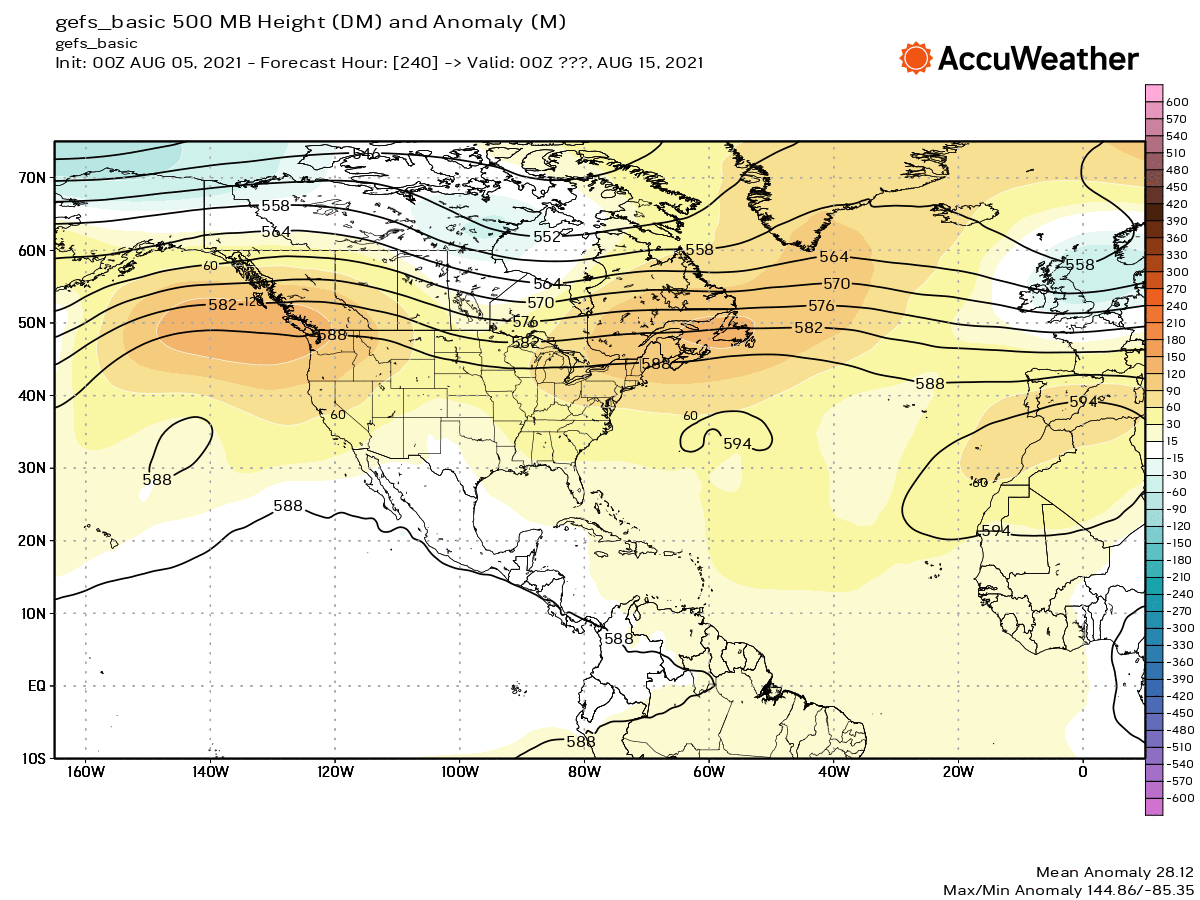
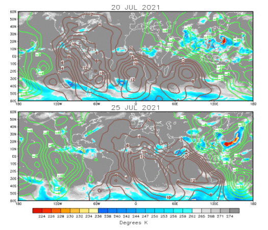
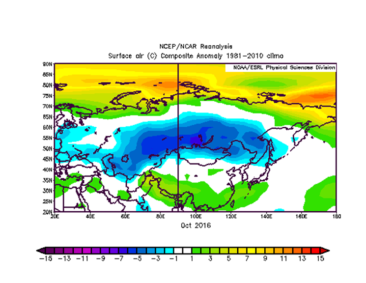
Synoptic and mesoscale conditions conducive to Type VI events have been established. Lashley and Hitchcock averaged data from 8 classic cases between 2003 and 2014 to produce synoptic scale composite anomaly charts. Like any lake effect snow event, Lavoie (1972) found the air-lake temperature difference to be the most important forcing mechanism for lake snows. Specifically, a lapse rate of at least 13ºC between the surface and 850mb is necessary for lake effect snows. That is no different for this Type VI case. In addition, all of the classic documented cases thus far have had a distinct 250mb and 500mb trough or closed low. Trough heights (particularly at 500mb) directly over the Great Lakes region are 180m below the climatological average (1981-2010). This points toward the need for strong upper dynamics yet weak upper flow to be present for a classic case to occur. The images above are the plots created by Lashley and Hitchcock to help identify these conditions. 500mb Geo potential height anomaly is plotted in the upper left. At 850mb, it is noted during these classic cases that lower than average heights occur to the southeast and greater than average heights to the northwest of the Great Lakes. This is seen in the above image on the lower left. This leaves nearly neutral pressure conditions over the northern part of the lake as the center of the 850mb trough axis moves E-SE. This creates relatively calm wind conditions at the time of development between 00Z-06Z over the northern part of the lake. In addition, behind this trough at 850mb, exists cold air that has been identified to be approximately 11K below the climatological average seen in the upper right image. So another ingredient for this setup being that cold, arctic continental air be pushing into the Midwest between mid and lower levels. This helps to create steep mid-level lapse rates which will allow the circulation to continue to grow once initiated. At lower levels, a surface trough perpendicular to the lake is present which moves south with an associated 925mb trough and vorticity maximum. This is likely a result rather than a cause due to the large amounts of surface convergence present in all of the classic cases. Off to the west of the lake surface, an arctic air mass pushes in over the Dakota’s with pressure readings 12mb above the climatological average which is a result of the passage of the strong upper trough seen on the sea level pressure graphic on the lower right.

THE CASE: FEBRUARY 18th, 2015

Starting overnight on the 17th and occurring into the early morning and day hours of the 18th, this case could arguably be another classic case to add to the list of archived Type VI events. This and other Type VI events have variable start times as the mesolow is not visible until the formation of the singe snow band on the lake side (west side) of its circulation. In this case, Gaylord, Michigan (KAPX) radar returns at 04Z show the initial signs of the mesolow moving W-SW.  By 06Z the circulation is moving S-SW down the shoreline. Make note of the looping gif image above to see this.

FIGURE 3

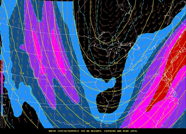
300mb Heights and Wind Analysis at 06Z

500mb

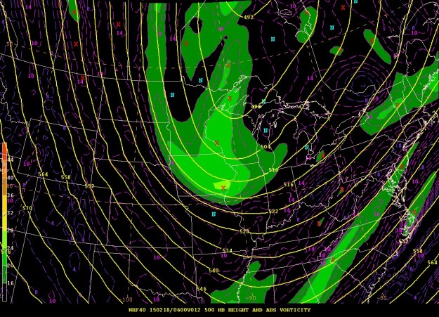
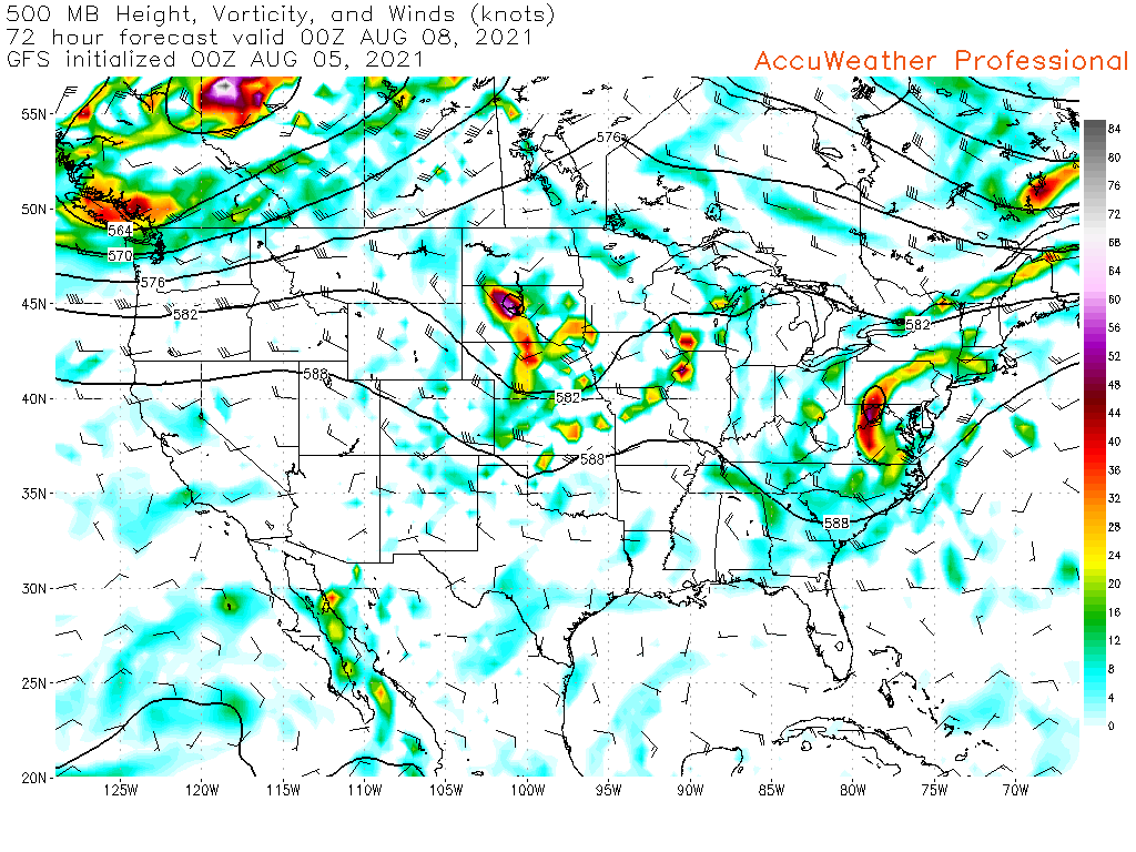
500mb Abs Vorticity Analysis at 06Z

At this 00-06Z time frame, synoptic conditions were conducive to a Type VI event. A 300mb trough axis was just to the west of Lake Michigan (note 300mb analysis above). Being close to the trough axis allowed wind flow aloft to be minimal with jet cores associated with this trough over the Dakota’s and a downstream jet core of 150 knots over the upper east coast of the United States. Winds directly over lake were between 25-35 knots at the 00-06Z time frame.

At 500mb, the trough axis is aligned nearly directly underneath the 300mb trough. This leads to the same wind flow set up with winds slowing as they approach the subgeostrophic wind zone at the base of the trough. Along the base of this trough is some curvature absolute vorticity which will act to increase vertical motion, but will not be the primary forcing mechanism for the event. It is simply important to note that forcing terms aloft are not working against the formation of this event. With the associated 500mb absolute vorticity maximum near the Iowa-Illinois border at 06Z (note 500mb figure above), the synoptic conditions will tend to increase vertical motion as the trough axis moves over Lake Michigan per positive vorticity advection pockets which increases tendency for vertical motion.

850mb

850mb Heights and Temp at 06Z

850mb heights and temperatures, pictured to the left, are what we would expect to see for a Type VI event. The base of the 850mb trough at 06Z is directly over the northern part of Lake Michigan with the axis extending down into Illinois. Continental arctic air is moving in behind this front with frigid 850mb temperatures of -30ºC to the northwest of Lake Superior and surface dew points nearing -20ºF in the same area (UCAR surface data). This will act to increase mid-level lapse rates as this frigid air mass moves over the sub-freezing lake which still has just above freezing surface water temperatures. Moving further down in the atmosphere, at 925mb, there is a broad trough which deepens as it moves over the lake between 00-06Z. Then at 06Z, it becomes easy to locate the position of an E-W orientated boundary which will follow the path of the surface circulation. Make note that the trough at 00Z is only present over the northwestern part of Michigan and then drops south and strengthens as the surface circulation strengthens. Before the occurrence of strong surface convergence, the 925mb trough is very weak which leads one to believe that the 925mb trough and vorticity strengthening is due to a stretching of the surface to 925mb layer which would be primarily caused by the convergence zone at the surface. The images for 925mb abs vorticity are attached below at 00Z and 06Z respectively.

925mb1

925mb Abs Vorticity at 00Z

925mb2

925mb Abs Vorticity at 06Z

This synoptic setup aids the formation of the surface low by increasing the tendency for vertical motion as stated above, but it is not the cause of this circulation. There is no subsidence, which is good, but there is also no significant vertical motion being caused by the 300mb, 500mb, and 850mb features. So there must be something on the mesoscale or microscale that is causing this circulation that we initially see at 04Z to form. In researching the progression of this event, it is the diagram below that describes the events that lead to the formation and movement of the low down the lake shore.

Picture1

Progression of events which lead to Type VI snowband formation

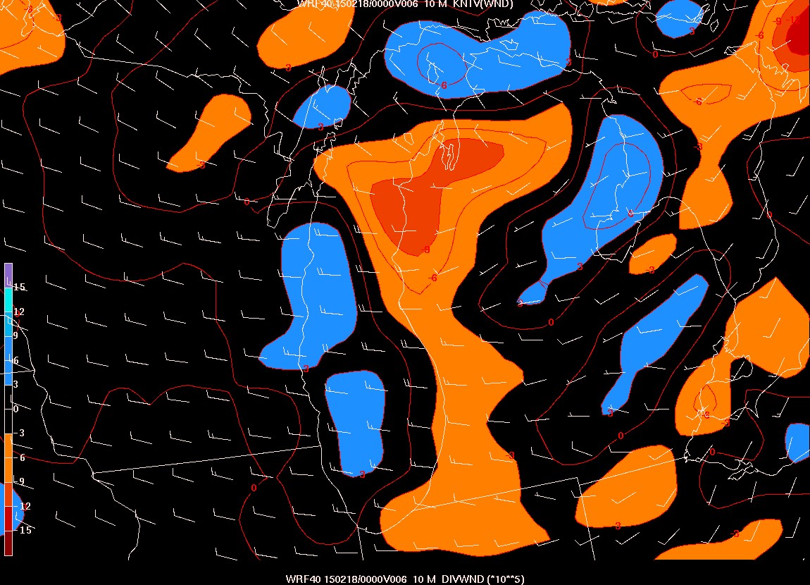
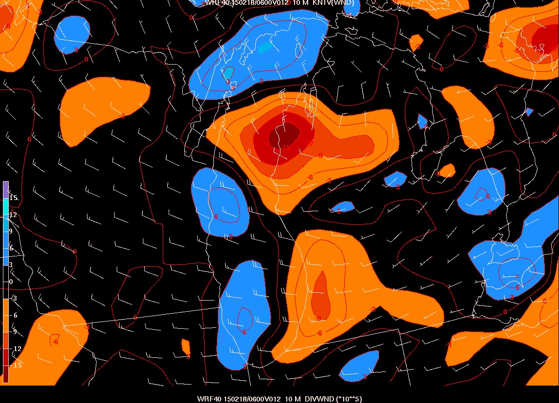
10 meter height surface winds can be found in Figure 6 and 7. The lake, which has a lower frictional coefficient than the land causes winds to accelerate over the water and then converge over the land due to an increased frictional coefficient and an increase in elevation. At 00Z, there are clearly winds accelerating over Lake Michigan (Note surface winds plot below). By 06Z however, we see that winds have continued to accelerate under the weak synoptic flow aloft. At 06Z, we see winds approaching the Sleeping Bear Dunes National Lakeshore (SBDNL) being between 12-16 knots or 14-18 mph. Over the land, winds are notably smaller in magnitude meaning that mass is being piled into the area near the shore. This is convergence. Any vector quantity with flow components u and v (north-south, east-west) can be decomposed into a rotating and non-rotating parts. With this, we should look at how divergence is calculated. This equation along with vorticity is listed below.

Capture


divergence types

Difference between speed and directional Divergence/Convergence

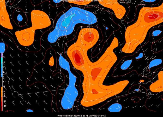
The calculation of divergence takes into account both directional and speed divergence (visualize difference in above figure). Convergence is the inflow of air into a layer or region and divergence is the opposite. Note that both speed and directional convergence is occurring due to the cyclonic turning of winds at 06Z (seen in the image below).

surfdiv00Z

Surface Divergence at 00Z

surfdiv

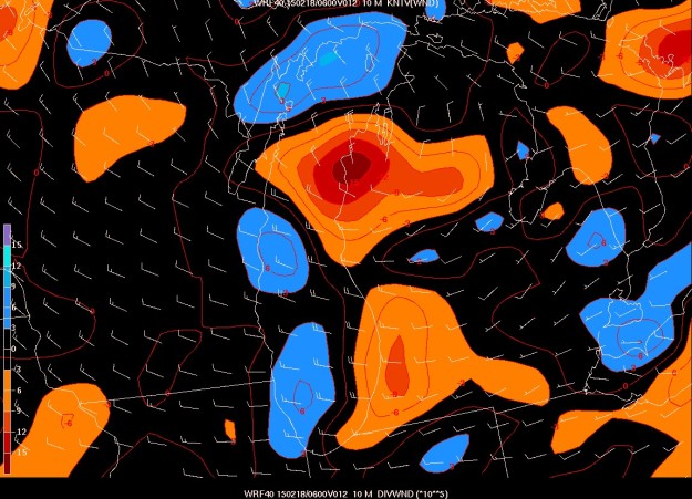
Surface Divergence at 06Z

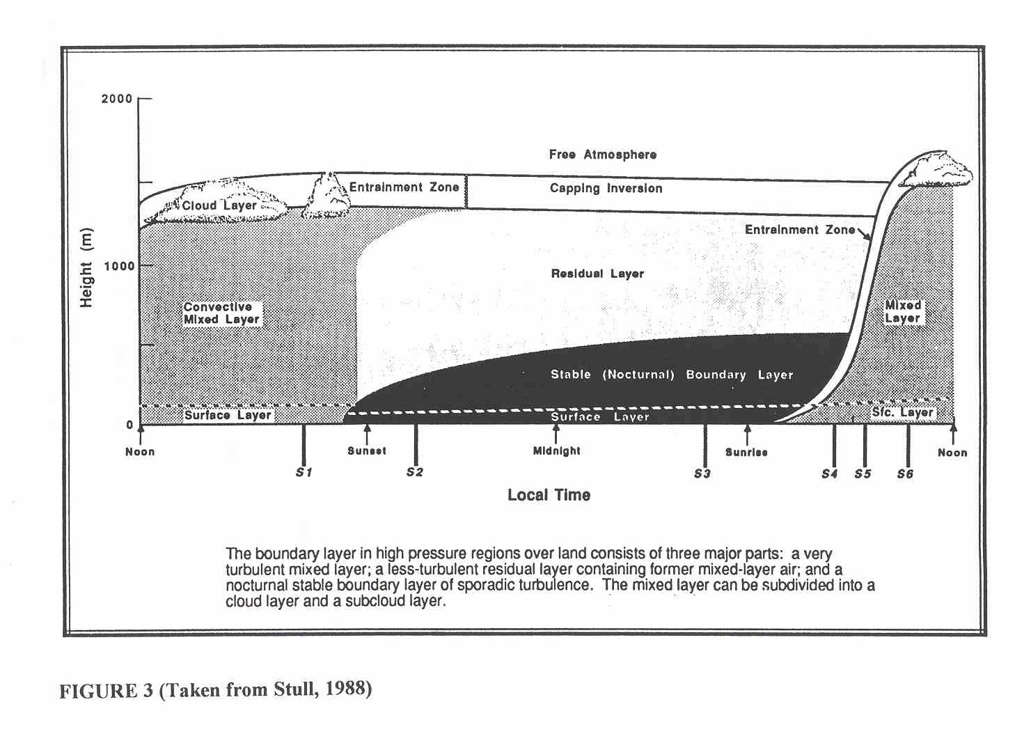
What this convergence then creates is vertical motion due to the influx of mass into the area. The progression of divergence/convergence at this initial formation time (00Z-06Z) can be visualized in the two above figures. The next step in the formation of this circulation is the creation of low pressure due to this rising motion. The tendency then is for air in the immediate surrounding area to move towards that area of low pressure. As air is forced into this small area of low pressure by the pressure gradient force, the Coriolis force acts to create the cyclonic motion seen in the circulation made visible on radar by the lake-side single snow band at 04Z. Roland B. Stull in An Introduction to Boundary Layer Meteorology studies convergent bands formed at the surface using a grid spacing of 2km. Therefore it needs to be recognized that we are studying a near boundary layer special scale event. It is difficult to study events on boundary layer special scales however.
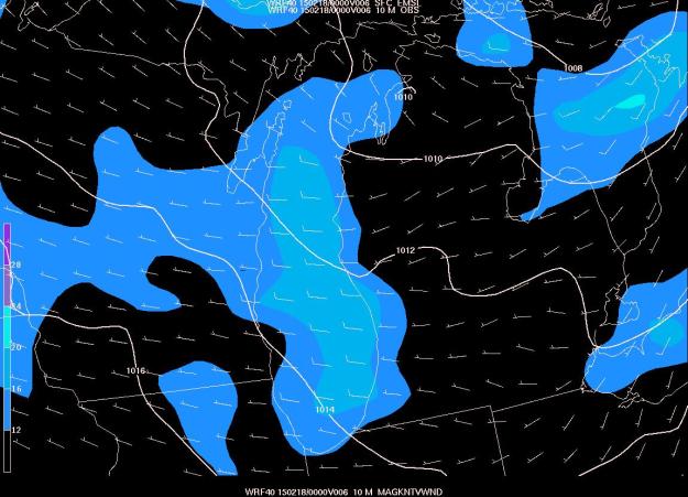
surfwinds

Surface Wind at 00Z

Surface winds

Surface Wind at 06Z

Starting at 06Z, the circulation starts to move in a more southerly direction. What causes this movement of the circulation down the lake is likely due to a couple of things. First, it has already been established that air accelerates over Lake Michigan due to a decrease in friction (note surface winds plot below). Therefore, this is also likely to be occurring as air moves around this small scale mesolow causing air to accelerate on the lake-side of the low and decelerate on the land side of the mesolow. In theory, what this would cause is the net movement of the circulation to be southerly down the shoreline. Forbes and Merritt (1984) point out that Type V events likely occur due to the curvature of the lake shoreline. This can be applied to the cyclonic curvature of the lakeshore from SBDNL to Holland, MI. From Holland, the curvature of the lake is than anticyclone as you head south down the shore. In many cases, we see the circulation move on shore near the Holland area indicating that this change in shore orientation might be a reason this circulation makes landfall in that area.

surfdiv12Z

Surface Divergence at 12Z

925mbvort

925mb Abs Vorticity at 12Z

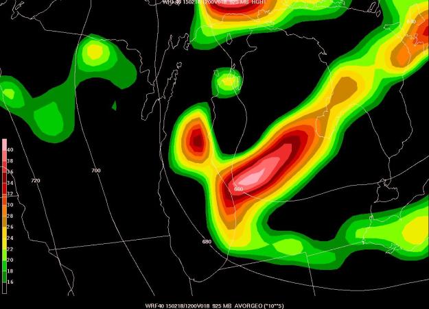
Between 06-12Z, we see the circulation grow significantly in many ways. Not only does the single snow band grow on radar returns and begin to wrap around the mesolow (note radar loop at beginning of post), but 925mb heights continue to drop and vorticity strengthens (note figure on right). Snow is now falling in the Grand Rapids area as well. Maximum surface convergence values are still correlated with the general position of the circulation which is located just off shore near Whitehall, MI (note below). At this point in the event, we start to see upper levels really begin to show signs of deep vertical motion with 700mb omega values up to -15 Pa/s (note below). In addition, strong mid-level lapse rates of up to -7.5ºC (only in the 850-700mb layer) are still present thanks to frigid 850mb temperatures (note below). This is where the weak synoptic environment aloft aids in the formation of this circulation. It’s possible that if there was stronger flow aloft that it would shear out the circulation or force it on shore earlier which makes it dissipate.

700mbomega12Z

700mb OMEGA at 12Z

850700mbdT12Z

850-700mb dT at 12Z


surfdiv18Z

Surface Divergence at 18Z

This event was in its ending stages between 12-21Z as a stronger pressure gradient associated with the upper trough moves in from the west. The upper trough axis is now to the east of Lake Michigan which means the jet core on the upstream side of the upper trough is starting to influence the area. What this ended up doing was forcing the circulation to move on shore. By 18Z, the circulation is pushed completely over land and the single band then starts to deteriorate (note radar loop at beginning of post). The analysis of lower levels show that strong onshore flow was still occurring. With this, strong convergent regions were still present in the SE corner of the lake (note figure on right). This area of convergence continued to produce a hybrid of Type I and II snow bands throughout the day on the 18th. However, 18Z 925mb heights and vorticity plots showed that the circulation was located near the NE corner of Indiana at that time (note figure below). Again, this is likely due to the increase in northwesterly flow from the increase in the pressure gradient over the area.

925mbvort18Z

A FRICTION EXPERIMENT

To test the hypostasis regarding the southward motion of the circulation. A second WRF run was submitted with altered land friction values. The land type of the Michigan shoreline was coarsely identified by plotting the land use map and eyeballing the land type. The land type 14 and 15 were changed to ¼ of the original value of .5 to make them .125. What would be expected to happen if this hypothesis is correct is that the circulation would progress to the east more quickly as air isn’t slowed over the land as much with lower friction coefficients. This didn’t happen. As a matter of fact, little change can be identified between the WRF run with regular and reduced land friction values which you can note below with the 06Z 10m divergence and wind plots.

The circulation progressed in nearly the exact same path that it did in the original WRF run. This can mean a few things. First and maybe most obviously is that differences in friction over the land and water play little role in the projection of the circulation down the shore. A second possibility is that this 40km model resolution is too broad to test this experiment with only approximately 6 grid points in the SBDNL to Holland, MI area. It might be that more grid points would increase the effects of friction on the circulation.

.25friction

Surface wind with 1/4 friction values at 09Z

regfriction

Surface wind with regular friction values at 09Z

Surface Divergence

Surface divergence with 1/4 the friction values at 12Z

frictiondiv

Surface divergence with regular friction values at 12Z

EVENT IMPACTS

This particular event did not have major impacts to southwest Michigan or northwest Indiana. A few reports of whiteouts were sent in on Twitter and snow totals were between 4” to 7.8” in the Benton Harbor area. Indiana hardly was effected by this event.   However, these events have caused major pileups on I-94 in the past, particularly on February 7th, 2003 (the first documented case) and January 23rd, 2014 (Lashley, 2014). Between the 2 of these events, there were 5 fatalities and numerous injuries due to large snowfall rates and whiteout conditions produced from Type VI events. In an analysis of previous events, these events can produce heavy snowfall rates of 1 to 3 inches per hour (Lashley, 2014).

FUTURE WORK / LIMITATIONS

The resolution of WRF which was used to generate all of the plots shown in this case study was 40km. Therefore, this circulation would not be sampled accurately using a model larger than 4km due to the fact that these circulations are around 2km in size (Stull, 1988). Future studies should look into creating a 4km reanalysis data set. With this, you should be able to pick up the circulation itself at the surface and the boundary layer parameterizations will be more accurate. A higher resolution model would also help study the influence of frictional differences on the direction the circulation moves. The study of the initial formation of the circulation is a boundary layer topic. With that said, it would be helpful (but maybe not cost effective) to get surface layer data of the strength of the land-lake breeze between 00-06Z. Along those same lines, what is so unique about the Sleeping Bear Dunes National Lakeshore area in the formation of wintertime mesoscale vorticities?

CONCLUSION

The proposed Type VI Lashley-Hitchcock snow band does not fit under any prescribed lake effect snow type. This is therefore a new type of lake effect snow. Starting overnight on the 17th and occurring into the early morning and day hours of the 18th, this case could arguably be another classic case to add to the list of archived Type VI events. The development of Type VI events starts with frigid W-NW surface winds flowing and accelerating over the seasonably warm lake surface temperatures on the northwestern part of Lake Michigan. Specifically in the Sleeping Bear Dunes National Lakeshore area. This causes horizontal convergence as mass and moisture piles up and mixes with cold, drier air over the shoreline. Not only this, but the presence of a surface frontal boundary creates directional convergence which further increases the convergence values. This creates significant vertical motion over the land breeze boundary (or area of peak convergence), which in turn forces an area of low pressure to occur over the area of maximum convergence. This allows the pressure gradient force and the Coriolis force to start cyclonic rotation in the area.  The further vertical development of the circulation is aided by rapid mid-level lapse rates and by the upper dynamic setup.

REFERENCES

Forbes, Gregory S., and Jonathan H. Merritt. “Mesoscale vortices over the Great Lakes in wintertime.” Monthly weather review 112.2 (1984): 377-381.

Holton, James R., and Gregory J. Hakim. An introduction to dynamic meteorology. Academic press, 2013.

Lackmann, Gary. Midlatitude synoptic meteorology. American Meteorological Society, 2011.

Laird, N. F., 1999: Observation of coexisting mesoscale lake-effect vortices over the western Great Lakes. Mon. Wea. Rev., 127, 1137–1141.

Lavoie, Ronald L. “A Mesoseale Numerical Model of Lake-Effect Storms.” Journal of the atmospheric sciences 29.6 (1972): 1025-1040.

Niziol, Thomas A., Warren R. Snyder, and Jeff S. Waldstreicher. “Winter weather forecasting throughout the eastern United States. Part IV: Lake effect snow.” Weather and Forecasting 10.1 (1995): 61-77.

NOAA : National Centers for Environmental Prediction. WRF Data Source. 3 Mar. 2015. Raw data. N.p.

Noone, David. “Circulation Theorem.” Colorado University. May-June 2015. Lecture.

Stull, Roland B. An introduction to boundary layer meteorology. Vol. 13. Springer Science & Business Media, 1988.

Turbulence in the Boundary Layer and Effects on Aviation Operations

When it comes to meteorology, not many people understand the complex diurnal evolution of the Boundary Layer (BL). Every day, the sun transforms the characteristics of the boundary layer into a well-mixed convective mass conserving machine. This process, along with others which I will address throughout this paper, make the study of the boundary layer very important. The study of the boundary layer is also important because we spend nearly all of our lives living in it. Forecasts for temperature, dew point, surface winds are all really BL forecasts. We also look at the BL in studying the production or dissipation of turbulent motion through a variety of terms that will be discussed. The study of turbulence presents many issues. How do we model turbulence? How do we differentiate turbulence from other large scale dynamical phenomena? How do we forecast turbulence in the real atmosphere? These are all questions that need to be considered. This turbulent motion or the deviations of the instantaneous mean wind flow (Panofsky, 1959) also causes many issues for aviation operations at airports and the surrounding terminal aerodrome where planes are coming up and down through the boundary layer. Everyday worldwide. According to the FAA’s website, 24 people were injured in 2013 due to turbulence experienced while in flight. In the last 10 years, 369 people have been injured in flight due to turbulence. Notice that no one has died due to turbulence! The encounter of turbulence can come with nearly zero forewarning which is how most of these injuries occur and is also why this is still such an active area of interest. It also however is extremely common, should it be that big of a deal?

In this post, I plan to review the production and dissipation of turbulence in the boundary layer with a focus on its potential effects on the aviation industry. I plan to explain what is objective in a subjective manner as to appeal to a larger, more lay audience. I will start with an introduction to the exciting subject of Boundary Layer Meteorology. From there I will discuss the characteristics of turbulence in the boundary layer as well as its production and dissipation. In the last section, I will discuss the implications of this turbulence on aviation operations in the boundary layer.

Hello Boundary Layer

In studying Boundary Layer during one of the busiest semesters of my college career, it has been a difficult subject to grasp. Take everything you learn in dynamics regarding the governing equations of the atmosphere and apply it to a much smaller time and grid scale. While you are at it, it is for all practical purposes mathematically impossible to model turbulence by following parcels like we do in Synoptic Meteorology. Therefore we apply statistics and utilize ensemble means to reduce the variance in understanding how turbulence progresses through the BL. Don’t let this scare you though! The idea of understanding turbulence and Boundary Layer processes is something that we still have yet to accomplish in classical physics. I plan to explain these things in a simple manner.

Before I go too deep however, let me make some brief introductions to the subject. Boundary Layer Meteorology is the study of how Earth’s surface effects the bottom 3km of the atmosphere over a short time period of roughly an hour or less. There are many meteorological processes which occur in the BL. Most notably including the fair weather cumulus clouds and stratocumulus clouds which includes fog. Ultimately however, the entire troposphere is influenced by changes in the characteristics of Earth’s surface (Stull, 1988). Thunderstorm formation, although not a BL process by itself, is heavily influenced by the BL through surface convection, cold pool interactions, outflow boundaries and various other processes which occur in the BL (Stull, 1988). How do conditions in the BL change? This is a broad question that someone just learning the subject might ask. It certainly isn’t an easy question to answer. Simply put though, change occurs in the BL due to the wind and changes in incident solar radiation. Now wind can be broken up into three categories: mean wind, turbulence and waves (Stull, 1988). I assume you understand what the mean wind is, it is self-defined. What I want to focus on is the occurrence of turbulence and how it is one of the most important transport processes in the BL. As defined above in my introduction, turbulence is the deviations of the instantaneous mean wind flow or the gustiness imposed on the mean wind flow (Stull, 1988). Differences in solar heating lead to the production or dissipation of turbulence and also lead to the different types of layers seen within the BL which do include but are not limited to the mixed layer, the residual layer, the stable boundary layer, the surface layer and a few others that I won’t mention for purposes of keeping this post short (Figure 1). These different layers are products of different thermal and flow properties. The mixed layer occurs in the afternoon when radiational convergence at the surface causes convection and therefore the vertical expansion of the BL as air warms, expands and then rises. The residual layer forms at sunset when surface heating is lost, turbulence begins to dissipate at the surface instead of being produced. However, the layer maintains characteristics similar to that of the mixed layer, but is now just separated from the surface. It is this layer that can instigate early morning thunderstorms. Moving into night time is when the stable BL forms as the tendency of air in contact with the surface will be to cool and become stable. The surface layer refers to the layer nearest to the surface. So this is anywhere from centimeters above the surface to a few meters. Some scientists define it as the bottom 10% of the BL. Turbulence is contained in all of these layers and in the next section I will go into more depth as to what the characteristics of turbulence are.

Figure 1 - The many different layers produced in the BL.

Figure 1 – The many different layers produced in the BL.

Turbulence

In doing some research for this paper, I have read a few cases of injuries experienced on planes where turbulence was the cause of injury. The one that flew out to me the most was a case of a flight from Rio de Janeiro to Houston which was forced to make an emergency landing in Miami due to 4 seriously injured passengers in August of 2011. 26 people were injured on this flight due to turbulence. That was not what stood out to me about this article though. What stood out to me was how the article highlighted that different meteorologists were saying different things regarding the presence of turbulence during the flight. Directly from the article, “Meteorologists differed on weather conditions at the time the Houston-bound plane encountered the turbulence just northwest of Puerto Rico.” I got the feeling from this article that people don’t recognize the physical complexity of turbulence and trying to predict its occurrence. Meteorologists are justified in saying this because turbulence is a very difficult phenomena to predict. You might as well be flipping a coin to see if it will occur in a particular area. Therefore, in this section, I will highlight turbulence and its characteristics in the BL to try to raise awareness as to the challenges that come with studying turbulence. Obviously, this will be focusing on the turbulence seen in the BL, but can also be applied to that seen in the free atmosphere.

Turbulence in the BL is different than turbulence aloft (free atmosphere) in the way that it is generated. Turbulence seen in the BL is primarily generated by forcings from the ground. Turbulence above the boundary layer is either generated in convective clouds or in the presence of jet streams where wind shear can create clear air turbulence. In the BL, production of turbulence comes from solar heating or thermals, frictional drag which causes wind shears (similar to CAT) and obstacles which then cause turbulent waves in the wake of flow downstream of obstacles. These different production methods lead to countless different sized circulations or eddies. In the mixed layer, eddies are generally elongated. It is this stretching in the mixed layer that actually is a source of instability for tornadic thunderstorms via vertical vorticity. In the SBL, eddies are generally more horizontally orientated. Hopefully this sounds strait forward. The BL is very much dictated by the influx of solar radiation. When that influx is lost, the elongation of the layer stops and subsidence occurs from above. Furthermore, turbulence is nearly continuous in the BL and more sporadic in the free atmosphere. This is due to the large amounts of turbulent production and dissipation seen throughout the day in the BL.

What is the challenge then? I’ve been talking up the complexity of turbulence this entire paper, why is that so? It comes down to the fact that turbulence is extremely difficult to describe and forecast mathematically. Turbulence generally occurs in circulations called eddies which I mentioned above. They are produced particularly in the mixed layer in the afternoon hours. It is these eddies that are transporting heat, moisture and momentum in the BL. Boundary Layer Meteorologists have developed stochastic methods to explore these turbulent eddies. That is, methods that deal with the averaging of the change of eddies over time since it is next to impossible to mathematically follow the them. To get average conditions means we need to measure something first, so how the heck do we sample turbulence? It is extremely difficult to sample these eddies by simply looking at a large area of space in time. For sampling turbulence and eddies, it is much easier to look at a specific point for a long period of time. This way, we don’t have to look at such a huge area where it is likely that conditions vary extremely from one side of the domain to the other. We don’t have the sensing capability or the funding to be able to put up enough sensors to do this. With this said, we then move to one of the most important topics covered in BL meteorology which is Taylor’s Hypothesis. This states that we treat turbulence to be frozen as it moves over our sensing device at a specific point for a large period of time. That is that it does not change shape or characteristics as it is passes over the sensor. This allows us to sample the turbulent eddies more effectively, but one must note that real turbulence is not frozen! Turbulent eddies are constantly evolving as they move over different types of land with varying meteorological conditions. Taylor’s Hypothesis allows us to think of eddies spatially based off of temporal measurements. So as you can maybe see here, the understanding Taylor’s hypothesis is a key concept to understand in BL meteorology.

Another challenge is the spectral gap. The spectral gap is a lack of variance in turbulence at the intermediate time or space scales (Stull, 1988). What this physically means is that at time scales around one hour, the spectral intensity is significantly less than that seen on large scales. This gap allows us to differentiate the difference between large scale (synoptic) phenomena like frontal passages and small scale phenomena like turbulence. Why is this an issue? This sounds fantastic! Well forecast models are calculated at time scales of about 1 to 3 hours depending on the model. This means they are calculating at a scale in the spectral gap. Scales larger than the time scale (synoptic scales) are resolved well but scales smaller than the model cannot be modeled and are approximated by parameterizations. This presents numerous errors in models which only grow with time.

Aviation Application

When people step on a flight, there is no better remainder of the difficulties in flight operation than the experiencing of turbulence. Whether that is just after liftoff or at 35,000 feet. Keeping our focus on the Boundary Layer, all of what I have stated regarding turbulence in the BL has a very important application to flight operations in the BL. Have you ever wondered why when you are climbing after takeoff or descending to landing the ride seems a little bumpier? This is turbulent eddies at work! Many passengers get made uneasy when this happens, but truth is, it’s completely normal (excluding the rare cases).

What are you experiencing though when you feel that sudden jolt? To adequately answer this question, we need to first answer how a plane is held in the air in the first place. Simply put, differences in pressure on either side of airplane wings are the source of lift on aircraft. Air moves faster over the top of the wing than the bottom which in turn causes lower pressure to occur on the top of the wing. This idea is also known as Bernoulli’s Principle. So if air is moving constantly over the wing, you would expect the aircraft to be flying steadily at a constant altitude. Turbulence though, as defined earlier, causes rapid increases in the mean wind to flow to move over the wings. This creates a rapid change in pressure which in turn causes the aircraft to react rapidly to equilibrate the pressure on either side of the wing. The result that you feel on the inside of the plane is that which causes your coffee to spill on your lap.

Planes are built to handle a respectable amount of turbulence. So pilots will generally think of turbulence more in terms of conveniency rather than a serious safety issue. Especially in the BL where passengers are generally instructed to remain seated until the aircraft reaches cruising altitude. What pilots and airport managers need to watch out for are wind gusts which could make landing exceptional difficult on rare cases. Windy days boast the mechanical production of turbulence at the surface so the BL on windy days is a turbulent mess. Especially near the surface where wind is trying to go around buildings and trees. Otherwise, on just a hot summer afternoon, you can expect a bumpy landing.

Conclusion

The study of Boundary Layer Meteorology is a field which needs a lot of work. Our knowledge and understanding of turbulence in the classical sense is very limited. This is mainly due to the complexity and nature of turbulence itself. We do not have an efficient way to measure turbulent eddies without making large assumptions. Once we have this data, we may try to forecast its progression through time based on stochastic models. This method works but is not as accurate in the long run as error is introduced through averaging and parameterizations in governing equations. The aviation industry and the people that utilize its services need to recognize the complexity of turbulence which every flight worldwide will run into at some point on its journey. Only on rare circumstances will you have turbulence severe enough to cause injury to passengers like that seen in the flight from Rio de Janeiro that made an emergency landing in Miami. This was caused by clear air turbulence too, not turbulence found in the BL. It is even rarer to find turbulence doing structural damage to aircraft since this is generally associated with thunderstorms and are easily spotted and avoidable. Raising awareness of these unknowns will help increase research on this topic. So fly informed!

Works Cited

Panofsky, Hans A. Atmospheric turbulence. No. SCR-118. Sandia Corp., Albuquerque, N. Mex., 1959.

Stull, Roland B. An introduction to boundary layer meteorology. Vol. 13. Springer Science & Business Media, 1988.

Catalano, Franco, and Chin-Hoh Moeng. “Large-eddy simulation of the daytime boundary layer in an idealized valley using the Weather Research and Forecasting numerical model.” Boundary-layer meteorology 137.1 (2010): 49-75.

Smith, Patrick. Turbulence: Everything You Need to Know. Patrick Smith’s Ask the Pilot: All Things Air Travel. < http://www.askthepilot.com/questionanswers/turbulence/>

Purdue classes…

Space Weather – The Meteorological Frontier

Talk about a subject that tilts heads, space weather is a rapidly growing field in science. I was first exposed to the subject in my Intro to Atmospheric Science class my freshman year at Purdue University. The professor, Dr. Ernest Agee pulled up two websites at the start of every class. The first being spaceweather.com and the other being the NCAR Real-Time Weather site. I had no clue why we were looking at space weather in that class. Weather in space? How does that work out!? Heliophysics… Sounds like a made up sci-fi term. These were thoughts that were running through my head. Little did I know how awesome the subject was! Four years later and I still look at the same space weather website nearly daily. The subject is intriguing, complex, dynamic, and is now becoming more and more economically important. Many people are turning to meteorologists for information about this subject and therefore many meteorologists are being recruited into this field which has been particularly significant for me as I start to consider career options. In this post, I plan to address a question that is commonly asked at me. What is space weather and why is it a growing field in science right now?

As defined by the Space Weather Prediction Center, space weather describes the variations in the space environment between the Sun and Earth. The study of space weather explains the multiple phenomena that can bring harm to satellite and Earth based infrastructure. Heliophysics is the branch of science that describes space weather (to make this post simple, this will be the only time I bring up the term heliophysics). It is no surprise that as we rely more and more on technology, we are relying more and more on satellite based communication and a dependable supply of electricity. GPS services, satellite based communication, astronauts and polar flight routes are just a few examples of services that can be interrupted by space weather.

Okay, so space weather refers to the phenomena that occurs between the Sun’s surface and the Earth. How does space weather work though? What are the phenomena? First off, I would like to comment on the consistency of the Sun’s energy output. This may seem elementary, but its important. The Earth is ALWAYS being bombarded with various wavelengths of radiation from the Sun. These include ultraviolet, visible and infrared radiation. Earth’s atmosphere manages to absorb and reflect much of the harmful UV radiation and much of what we experience on Earth’s surface is of visible wavelengths with a minimal amount of infrared radiation. Note figure 1 one showing the distribution of radiation we see on the surface of Earth. The Sun doesn’t go to bed at night and it doesn’t take naps in the middle of day behind cloud cover. Its ALWAYS present and thank goodness that it is! It is this radiation from the Sun that allows the existence of life on Earth.

Figure 1 // Spectrum for Solar Radiation on Earth. Note that visible wavelengths has the highest irradiance (or flux of energy per unit area).

Figure 1 // Spectrum for Solar Radiation on Earth. Note that visible wavelengths have the highest irradiance (or flux of energy per unit area).

Going off this idea that the Sun is ALWAYS spewing energy in all directions. The Sun’s outer atmosphere also releases energy in the solar wind, large amounts of radiation in solar flares and magnetic fields and plasma with coronal mass ejections (CME’s).  All 3 of these processes are the main phenomena that make up space weather.

The solar wind is a continuous out flowing of electrons and protons in the form of plasma from the Sun’s surface. There are also embedded magnetic fields with this plasma which will be very important when looking at how the solar wind will interact when it collides with Earth’s magnetic field. The solar wind varies in speed and density based on surface conditions of the Sun (look into coronal holes). The solar wind alone has the power to spark auroras and geomagnetic storms if its speed, density and magnetic field direction are working together.

Figure // Shown above is the latest forecast of conditions in the solar wind, as predicted by the WSA-Enlil model from the SWPC.

Figure 2 // Shown above is the latest forecast of conditions in the solar wind, as predicted by the WSA-Enlil model from the SWPC website. I include this because it allows one to visualize how the solar wind travels from the Sun outward into space.

A solar flare is another process that powers space weather. A solar flare is a large release of radiation from the surface of the Sun and are commonly associated with CME’s which will be covered in the next section. A solar flare releases extreme amounts UV radiation and X-rays thanks to a re-connection of magnetic field lines on the Sun. Its this process that causes radio blackouts on Earth. Though it may seem like radio usage is decreasing, it is still a widely used technology by the military, air traffic controllers and various emergency response organizations.

Figure 2 // An X-class solar flare on July 6th, 2012.

Figure 3 // An X-class solar flare on July 6th, 2012.

Last, but certainly not least is the Coronal Mass Ejection (CME). The Sun produces an UNBELIEVABLE magnetic field from the amount of energy that is being produced from its core. On the surface (the corona), these magnetic field lines tend to get tangled and twisted with huge amounts of energy being transported by extreme convection. When this happens, potential energy builds until this large gradient is released in the form of a CME. Nature always wants to be in equilibrium, even on the Sun. With this said, CME’s contain magnetic fields and plasma and spark enhanced geomagnetic storms and auroras on Earth. Below, you will find a video showing a CME eruption on March 14th of this year.

Figure 2 // An image from SWPC that summarizes the locations of space weather processes.

Figure 4 // An image from SWPC that summarizes the locations of space weather processes. This image is a dramatization and is not to scale.


Since the Sun is constantly releasing these flares, ejections, wind and what not, why don’t we see more geomagnetic storms and auroras? Much like how the ozone layer protects us from harmful UV radiation, Earth’s magnetic field protects us from the solar wind and CME’s. Earth’s magnetic field can be simply visualized like that of a magnet. Its shape changes like that seen in Figure 4 thanks to the pressure of the solar wind. The solar wind causes a compression on the day side of Earth and stretching on the night side. Its Earth’s magnetic fields that explain why the auroras and geomagnetic storms occur most frequently at the poles! Energy released in CME’s and contained in the solar wind travel along the magnetic field lines of Earth which are directed to the poles. It is here that this energy excites oxygen and nitrogen molecules in the ionosphere. When these molecules return to their steady state, they release energy in the form of light! This creates the aurora. A geomagnetic storm is a large disturbance in the magnetic field of Earth. It is CME’s that most often cause this large disturbance. These storms cause heating in the ionosphere which can cause errors in GPS positioning information, extra drag on satellites in low orbit and geomagnetic induced currents in the power grid and pipelines. Not only this, but storms can also expose people and flights in polar regions to unhealthy amounts of radiation. If given a warning in advance, companies can take precautions to save millions and even billions of dollars in damage.

The Sun is a fusion masterpiece. We have seen all of these processes described above for thousands of years. Its only been in the last two centuries that people have begun to study and understand what is going on. Today, greater than ever, we look to understand the variations in the Earth-Sun space environment to protect life and property. It is why this field is growing so quickly. Forecasters at the Space Weather Prediction Center take analysis data from satellites and models to predict if and when a particular storm will impact Earth. If they issue a warning, this allows companies to take the necessary precautions to protect the power grid, drilling and satellite operations, and astronauts in space. They just released a new website thanks to the increasing demand from companies and even the general public. The more we rely on satellites, the more we explore into space, the more we will need to understand and predict space weather.

Science rules!

Joe Bauer


For more information on space weather, explore the SWPC website and this website.

Further reading // where I got my knowledge:

Howard, T. A., Webb, D. F., Tappin, S. J., Mizuno, D. R., & Johnston, J. C. (2006). Tracking halo coronal mass ejections from 0–1 AU and space weather forecasting using the Solar Mass Ejection Imager (SMEI). Journal of Geophysical Research: Space Physics (1978–2012)111(A4).

Liu, Y., Thernisien, A., Luhmann, J. G., Vourlidas, A., Davies, J. A., Lin, R. P., & Bale, S. D. (2010). Reconstructing coronal mass ejections with coordinated imaging and in situ observations: Global structure, kinematics, and implications for space weather forecasting. The Astrophysical Journal722(2), 1762.

Lanzerotti, L. J. (2001). Space weather effects on technologies. Space Weather, 11-22.

Schwenn, R. (2006). Space weather: The solar perspective. Living Reviews in Solar Physics, 3(2), 1-72.