
INTRO
An historic winter occurred in much of the Pacific Northwest extending into California, and under a neutral El Nino Southern Oscillation (ENSO) pattern to boot! Not many long range forecasters would have given much weight to a forecast that was outputting the Pacific Northwest and California having a hectic winter back in the fall, but here we are looking back on the season and what a crazy ride it has been. To give you an idea on just how crazy a ride it’s been, let’s take a look to the record charts. To start, Nevada and Wyoming as a state had their wettest winter seasons on record (December-February). California had its second wettest winter on record (184% of normal precipitation) with the only other winter ahead of it being the El Nino winter of 1969. The drought in California was annihilated in the month of February with multiple atmospheric river induced storms moving over the region. The drought ridden state entered the month with 51% of it being under a drought designation. By the end of the month, only 9% of the state was under a drought designation with many regions seeing catastrophic flooding! Speaking of February, this specific month was a particularly active one for much of the West. Portola, California, a city nestled in a valley amongst the Sierra Nevada Mountains, received 12.36 inches of precipitation in February. This broke all previous records in place in its 102 year history of recording data. Bonners Ferry in far northern Idaho also received its record amount of precipitation with records started in 1907! Figure 1 below shows the distribution of precipitation as a percent of average which you’ll note a large portion of the west was above normal. Along the Sierra Nevada in February, snow water equivalent values were 150-200% of their normal values for February. Much of the winter out west was truly very active with much of the region seeing above normal precipitation. Take a look at figure 2 for a few highlighted station records with those graphics being put together by the National Centers for Environmental Information.
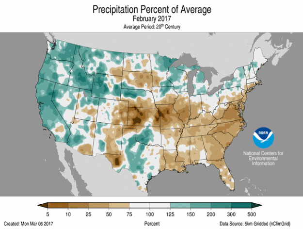
Figure 1: Percent of Normal Precipitation for the month of February

Figure 2: Review of observations near record this winter.
OUTLINE
With the wide area of above average precipitation out west this winter, this leads one to ask the question (at least it leads me to ask the question); how did this happen? Especially with a neutral to even weak La Nina ENSO pattern, things didn’t look like they were going to do more than an average winter before the season began. Well, first off, there is more that needs to be looked at in long range forecasting than just the ENSO pattern. There are a plethora of other climate teleconnections that can be studied and analyzed when trying to come to a consensus on a long range forecast. A simple google search of these phenomena will pull you up a variety of utilities to help one learn about these connections. I will draw more on the specific connections that were crucial to the west winter in the sections to come, but for now I return to the question at hand; how did this happen? To answer this question, my plan is to walk you through a specific event that impacted California from February 16th through the 18th of 2017. From there, we will take a look at the Pacific Sea Surface Temperature (SST) anomalies, their impact on the storm itself and how they influenced the rest of the winter. Lastly, I will conclude on how this setup can be recognized for seasonal forecasts. This will include an analysis on teleconnections and upstream conditions from this past winter.
SETTING THE SCENE
To understand the significance of the February 16th through the 18th event, one must be aware of what happened leading up to February 16th… It was bad. My shifts at AccuWeather were crazy busy only because the western half of the country was so active. Multiple waves of energy crashed into Northern and Central California from February 1st through the 10th. This created abnormally high amounts of precipitation from the northern central valleys to the Coastal and Sierra Mountain Ranges. I’m not talking just a few inches above normal either, areas centered on Portola were 9-12 inches above normal only half way through the month as depicted by figure 3 below. Farther south in California wasn’t as bad for the beginning of February, a little rain did manage to make it to southern California on the evening of the 10th but for the most part southern California was thirsting for some rain going into middle February with much of the region under moderate drought conditions which you can see below in figure 4.
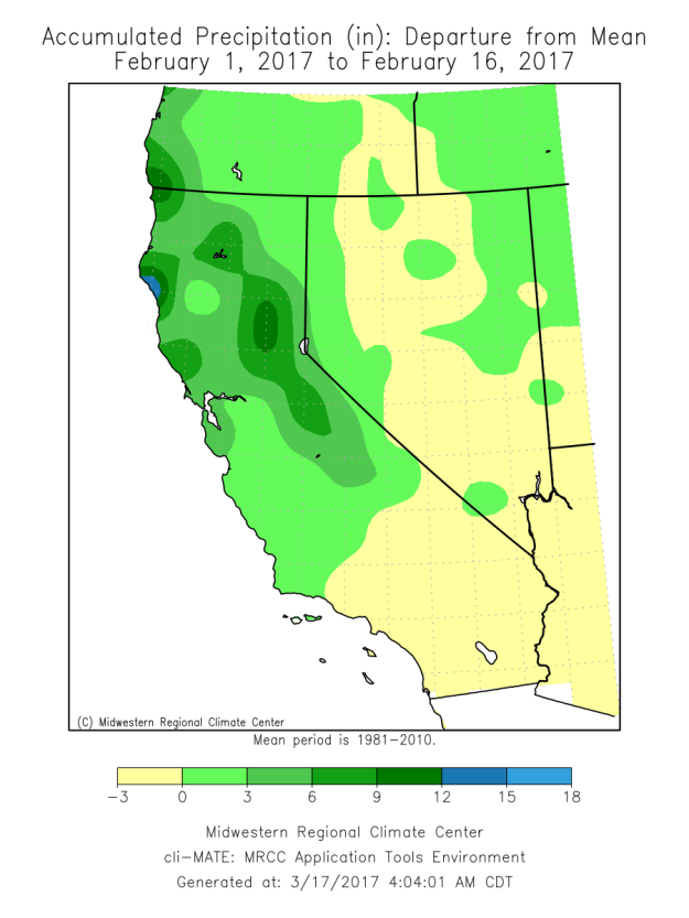
Figure 3: Departure from mean precipitation from the 1st through the 16th.

Figure 4: Drought monitor for the end of January.
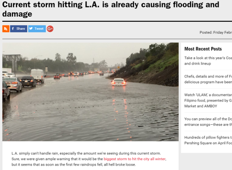
From February 10th through the 15th, dry weather moved into all of California which made for a nice break within a stormy pattern. Although no precipitation was falling, runoff from excessive mountain rain caused significant issues surrounding the Sierra Nevada. This was heavily publicized on Portola (picture 1) and the Oroville Dam (picture 2). The surrounding cities in the valley adjacent to the Oroville Dam were actually evacuated in fear that the dam would fail and deal catastrophic flooding damage to areas across the central inner valleys just southeast of Sacramento. This made national, continuous news coverage for multiple days surrounding Valentine’s Day. I actually remember coming into work on Valentine’s Day with news coverage saying that the dam could break at any moment. It was a rather intense situation waiting to see if the dam would break and the potential warnings we would have to issue. Meanwhile, all of this unfolding while another Pacific storm system was brewing in the Central Pacific. *insert Jaws theme music here*
-

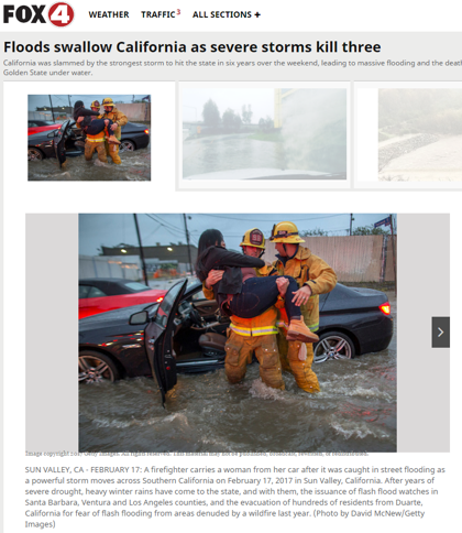
Picture 1: Firefighters responding to the widespread flooding in Portola. Multiple water rescues occurred.
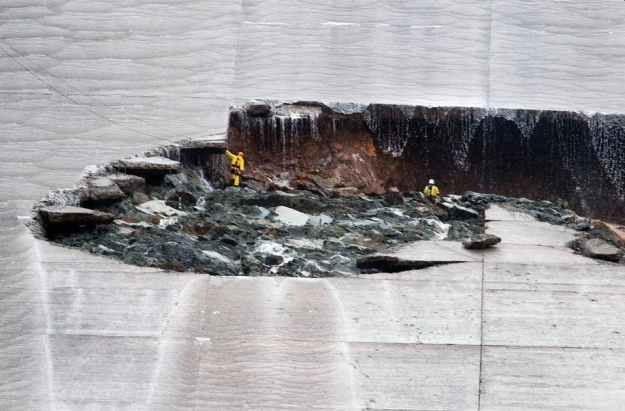
- Picture 2: Crews investigating the extent of damage to the Orville Dam spillway on the 10th.
THE CASE
Leading up to February 16th, model output was consistent on there being another large event for California which would last from February 16th through the 18th. Most media outlets were already hyping up the next round of rain while they were covering the flooding already occurring. The spatial and temporal variability in where the strongest rain and snow would occur with the next wave was high which led to forecasts shifting around quite a bit leading up to the event. As usual, I think too much weight is put on the quantitative precipitation forecast (QPF) output by deterministic models. Especially when forecasting along the west coast in these scenarios, numerical weather models will not do a good job. I repeat… they will not do a good job! This is mainly due to the atmospheric conditions over the Pacific Ocean not being sampled well due to a lack of surface observations and available soundings. We do have decent satellite coverage which helps out but overall the data that is being ingested into models as initial conditions over the Pacific is largely parameterized which leads to errors in the modeled forecast. Hopefully, GOES-16 (a new kick butt geostationary satellite) will aid in creating better surface and upper air analysis for models to utilize. Until then though, west coast forecasting is a great place for a human forecaster to shine (yay me and other fellow meteorologists!). With the human aspect of forecasting in these scenarios, I say that knowledge of upper air conditions (especially 700-500 mb) and sea surface temperature anomalies become increasingly important to determine where the heaviest rain or snow will occur. I’ll demonstrate this later in the post. With that being said, let’s take a look at what models were outputting for this event.
500 mb
A predominant zonal pattern was in place across the Northern Pacific for the days leading up to this event. Over the Central Rockies, a distinguishable ridge was present. The 12z upper air analysis on the 15th (figure 5) showed a narrow 70 to 115 knot jet extending from Japan to the northwest US and western Canada. This jet would quickly amplify with the 12z analysis on the 16th (figure 6) as multiple embedded filaments of vorticity sped through the predominant zonal jet. By 12z on the 17th (figure 7), multiple 500 mb waves are lining up under geostrophic flow across the Northern Pacific with large amounts of quasi geostrophic accent occurring in southern California. Meanwhile, the ridge controlling the Central Rockies, although it broke down slightly in response to wave that moved over the top of it on the 16th, remained entrenched. This pattern made for an active pattern for the Pacific Northwest while also being conducive to cut off low pressure systems sweeping underneath the upper ridge. Upon studying GFS and European model data 48 hours before the event (Figure 8-9). Minimal differences were seen between the GFS’s and European’s 500 mb model out. The GFS actually ended up verifying slightly better with the upper low not closing off until after 00z on the 19th. The Euro had it cut off by this time. This is why it is important to study upper air conditions first when preparing a forecast because most models within 48 hours do a, for all intensive purposes, a near perfect job on upper air conditions. This isn’t the case with modeled surface conditions.
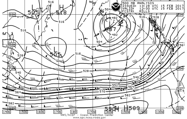
Figure 5: 500 mb Analysis on 12z February 15th by the Ocean Prediction Center
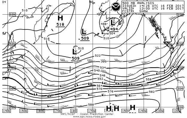
Figure 6: 500 mb Analysis on 12z February 16th by the Ocean Prediction Center

Figure 7: 500 mb Analysis on 12z February 17th by the Ocean Prediction Center

Figure 8: European modeled 500 mb conditions valid 00z on Saturday the 18th and initialized on 12z on Thu the 16th.

Figure 9: GFS modeled 500 mb conditions valid 00z on Saturday the 18th and initialized on 12z on Thu the 16th.
700 mb
In pulling up 700 mb relative humidity plots, one could very well visualize the river of moisture which was setting up to the southwest of the California coast at 12z on the 16th. More reasons to be familiar with your upper air conditions! Cough cough**. The images below (Figure 10-11) show the Euro and GFS output for that hour. These are the modeled initialized conditions. Both the GFS and Euro handled the moisture with a fair amount of agreement except that the GFS has a bias to saturate more of the layer than the Euro does. Overall though, the two models highlighted similar areas and values of RH. I wasn’t able to find any analysis data to verify initialized model data.
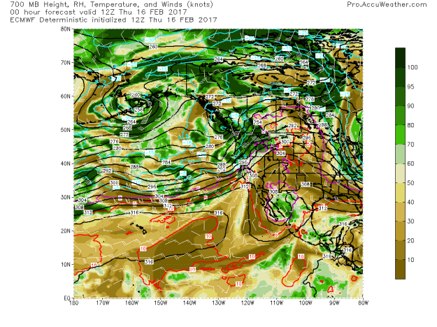
Figure 10: European modeled 700 mb conditions valid 12z on Thursday the 16th and initialized on 12z on Thu the 16th.

Figure 11: GFS modeled 700 mb conditions valid 12z on Thursday the 16th and initialized on 12z on Thu the 16th. Comparing GFS/Euro, you can see GFS has a bias to saturate more of the layer than the Euro does. Hmmmm.
850 mb
In looking at precipitable water (pwats) and 850 mb winds, one could even better visualize the strength and depth of the atmospheric river that was setting up back to the southwest of California. On the morning of the 17th, 1+ inch pwats moved into southwest California. It was at this time frame that the heaviest rainfall was moving over southwest California. These high pwat values would remain in the region through 00z on the 18th when the system finally shifted east into the Desert Southwest (See figures 12-13 below). However, with a whole day of 1 inch pwats in the area, southwest California was bound to pick up some significant precipitation.
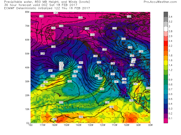
Figure 12: European modeled 850 mb conditions with precipitable water filled. Valid 00z on Saturday the 18th and initialized on 12z on Thu the 16th. This was around the end of the heaviest rainfall in SW California.

Figure 13: GFS modeled 850 mb conditions with precipitable water filled. Valid 00z on Saturday the 18th and initialized on 12z on Thu the 16th. This was around the end of the heaviest rainfall in SW California.
Surface
By 12z on the 16th, surface cyclogenesis had already occurred northeast of the Hawaiian Islands with a closed surface low of ~1000 mb (see figure below). This system would continue to deepen as it moved eastward, making landfall just south of Sacramento on the evening of the 17th as a seasonably powerful 984 mb low (see figure below). Shortly after this early on the 18th, the low occluded and turned into an open wave by the evening of the 18th. Its associated 500 mb shortwave was moving nearly completely meridional and parallel with the coast, the surface low followed suit and remained hung up on the coast through the 18th (see 00z 19th output below). Although the low was occluded and weakening by this point, this still allowed for heavy, warm sector rains to continue in southern California.
What Ended Up Happening
With all these parameters in place, a record setting rain event unfolded for much of California from 00z on the February 16th through the afternoon of February 18th. Precipitation spread from northern portions of the state to southern portions throughout the course of the event as the system tracked east-southeast along the coast (see radar loop below). Precipitation did manage to linger in the northern central valleys throughout this event due to sufficient moisture return from the Pacific and the surface low remaining just off the coast. You can visualize with the modeled surface plots above. The European ended up doing a little better with the track of the surface low remaining along the coast. That said, much of the coastal range saw 2 to 4 inches of rainfall with northwestern California seeing locally higher totals to 6 inches. The southwest coastal mountains, focused from Santa Barbara to north of Los Angeles saw as much as 10 inches of rainfall with the valleys seeing anywhere from 2 to 5 inches of rainfall. The northern central valleys of California saw 2 to 4 inches with the southern valleys seeing 0.5 to 1 inch of rainfall being heavily shadowed from the mountains to the southwest. Rainfall of this spatial and temporal magnitude made for potent and widespread flooding. Take a look at rainfall totals below (figure 14-15) National headlines again were made with the coastal range, the northern central valley and southwest California all seeing significant flooding.
Composite Radar Loop: 00z on the 16th through 15z on the 18th.

Figure 14: Total accumulated rainfall between February 16th and 18th.

Figure 15: Total accumulated rainfall zoomed on Southwest California between February 16th and 18th.
An Active Month for the West Explained
As I’ve hopefully made clear in this post, the spotlight was on much of the West (especially California) for the entire month of February. From the Oroville Dam in the beginning of the month, to the heavy, flooding rains in the middle of the month, to what seemed to be continued heavy snow over the Sierra Nevada, to say the west was under an active weather pattern this past winter would be an understatement. Going back to the records that were mentioned in the introduction, Portola, CA broke all records with 12.36” of precipitation through the month. Records for Portola started back in 1915. Venado, CA located amongst the coastal range north of San Francisco, picked up an incredible 37.45” with its previous record being 19.24”! In the Sierra Nevada Range, Tahoe City received 16.66” of precipitation which was its 2nd wettest February on record. This was 293% of its normal precipitation! Shoot dang. The Sierra Nevada saw snow water equivalent values 150-200% of normal for February. The drought was also gone! At the start of the month, 51% of the state was under a drought designation with only 9% having any drought designation by the end of the month. Idaho and Wyoming also saw a very wet month of February. For the whole winter (Dec.-Feb.), Nevada and Wyoming saw their wettest winter on record! Although the focus of this write up is the event which impacted California on February 16th through the 18th, I would like to use this event to help summarize the entire winter out west as it was these kind of systems which continued to occur through the winter. Let me explain.
So it’s about time for some explanations. It is hypothesized, by me and a few other colleges that I work with, that teleconnections, the upstream fall conditions on the Asian continent and sea surface temperature (SST) anomalies across the Pacific were to blame for the development of events in February for California and really the active west winter as a whole. Lets finally take a look into teleconnections as promised from earlier. The three teleconnections analyzed for this blog post were the El Nino Southern Oscillation (ENSO), the Pacific Decadal Oscillation (PDO) and the Pacific North American (PNA) teleconnection. As mentioned in the introduction, the ENSO pattern was neutral for this winter which allowed for other teleconnections to shine. The PDO was neutral to slightly positive for the whole winter. A positive PDO causes a zonal distribution of SST anomalies across the central Pacific with water just off the West Coast of North America being normal (neither anomalously cold or warm). This pattern can in turn promote a strong zonal jet stream across the Pacific Ocean due to the thermal wind. This said, any system that develops over the Pacific would have a clean shot at riding this jet stream right towards the western US. The PNA is a widely variable teleconnection which generally oscillates back and forth from negative to positive on the course of a week or so. However, when you average the PNA index over the course of the 2017 winter (December through February), it is slightly positive at 0.08. At the start of the event on February 16th, the index was very positive (1.4) and made a transition to nearly neutral (0.3) by the end of the event. A positive PNA is associated with above average 500 mb heights over the Intermountain West. This puts the upstream side of the ridge, where upward atmospheric motion occurs along the west coast. How convenient, mmm yes. This allowed systems throughout the winter to either slide up over the ridge towards areas like Bonners Ferry, ID (far northern Idaho) which saw its record amount of precipitation, or slide underneath the ridge like our case on February 16th through the 18th. That said, we need to dwell a little more on the zonal distribution of SST’s.
What caused this zonal distribution of SST in the Pacific throughout this winter? Certainly the PDO reflected this zonal distribution, but the PDO itself wasn’t the cause but rather just a measure of the distribution itself. So it is proposed that upstream conditions in the fall of 2016 in eastern Asia influenced and cooled SST across the northern Pacific. From October to November, anomalously cold conditions were in place across much of northern Asia (images below from the NWS show global temperatures with the ONLY area of significant below normal temperatures being in northeast Asia… also view figure 16 for reanalysis data). Looking at 300 mb winds across this area for the same time, we see anomalously strong westerly winds, pushing this cold air across the northern Pacific (figure 17) and in turn causing the anomalously cool SST in the northern Pacific to develop in October and expand juristically in November (see grouping of images below to visualize this… its pretty incredible really. I have the previous winters (2015-2016) SST anomalies attached as well for comparison).


Figure 16: Reanalysis data of surface temperature anomalies in October of 2016 of the Asian Continent. Note large area of below normal temperatures!!

Figure 17: Reanalysis data of 300mb zonal wind anomalies in October to November of 2016 over the Asian Continent. Note large area of above average winds in northeast Asia and northern Japan into the Northern Pacific.


Conclusion
An historic winter occurred out west during the 2016-2017 season. It seemed that there was never an end in sight with storm after storm rolling into the west throughout the winter months. In analyzing one storm from February 16th through 18th, 2017, highlighted forecast parameters were handled well by both models (EURO and GFS) and did not shift much within 48 hours of the event. Especially the upper air features which were handled very well. As usually the case though, the forecast challenge appeared to be mesoscale in nature. Namely where the best upslope flow caused enhanced precipitation along the coastal mountains whos orientation was normal to the southwest flow aloft. The hardest hit areas included the central Sierra Nevada, the California coastal mountain ranges and southwest California, especially in and around Santa Barbara and Oxnard, CA. Record and widespread flooding was seen across many of these areas, busting the drought that had a stranglehold on California for years. In short, this active pattern was caused by sea surface temperature anomalies in the northern Pacific Ocean. Specifically colder anomalous waters to the north with warmer waters to the south. This gradient promoted prime conditions for continued surface cyclogenesis to occur (much like the classic polar front theory). The stronger, prolonged systems (like Feb 16-18) commonly developed under the aid of a shortwave aloft. So looking at upper levels, an El Nino-esque Pacific jet stream extended (nearly zonally) from Japan to the northwest US coast for much of mid-February. Becoming very amplified at times (Feb 16-18). The sea surface temperatures anomalies in the Pacific were caused by an anomalously cold air mass (5º below monthly normal!) which developed over eastern Asia extending east through northern Japan. At the same time, an anomalously strong upper jet stream was in place to advect this air over the Northern Pacific Ocean. Sea surface temperatures in the northern Pacific began responding to this air mass in October, but especially expanded in November before temperatures in East Asia rebounded in December. These cool sea surface temperatures slowly drifted eastward across the Pacific throughout the winter, allowing storm systems to ride along the gradient towards the west coast the United States.
Going forward for long range forecasting, less weight needs to be put on the ENSO especially when it is neutral. Look to sea surface temperature anomalies and how the jet across the Pacific is setting up and what is changing these two variables. I recommend looking into how the fall season in eastern Asia transpired as in this past 2016-2017 winter it looked to play a pivotal role for the Western US.
Feel free to let me know if you have any questions or comments!

http://www.fox4now.com/news/news-photo-gallery/floods-swallow-california-as-severe-storms-kill-three
